Figure gallery
Every figure the package draws, on real data, with what each one is for
Each of these is produced by test/run_all.py against the public test corpus and copied into test/output_figures/gallery/. They are regenerated from the code, so a figure here is what the current version actually draws – not a screenshot taken once.
The caption under each image is the same text the figure prints beneath its own axes. There is one copy of it, in colorscheme.yaml, so the website and the PNG cannot drift apart. The same file’s ui block sets the colours and fonts of both HTML reports and of this site, so a figure, a report and a page of the documentation share one palette: Okabe-Ito for data, because group membership is carried by hue alone and has to survive colour-vision deficiency, and the logo orange, in a darker shade where it is text, only for links and controls.
docker run --rm -v "$PWD:/work" -w /work falconage:1.0.0-cpu \
  python test/run_all.py
Which dataset each figure comes from, and why that one was chosen, is recorded in SOURCES.md.
Start here
One figure for the question everyone actually has: which of these algorithms detects anything.
Clock atlas: every algorithm across every pooled study
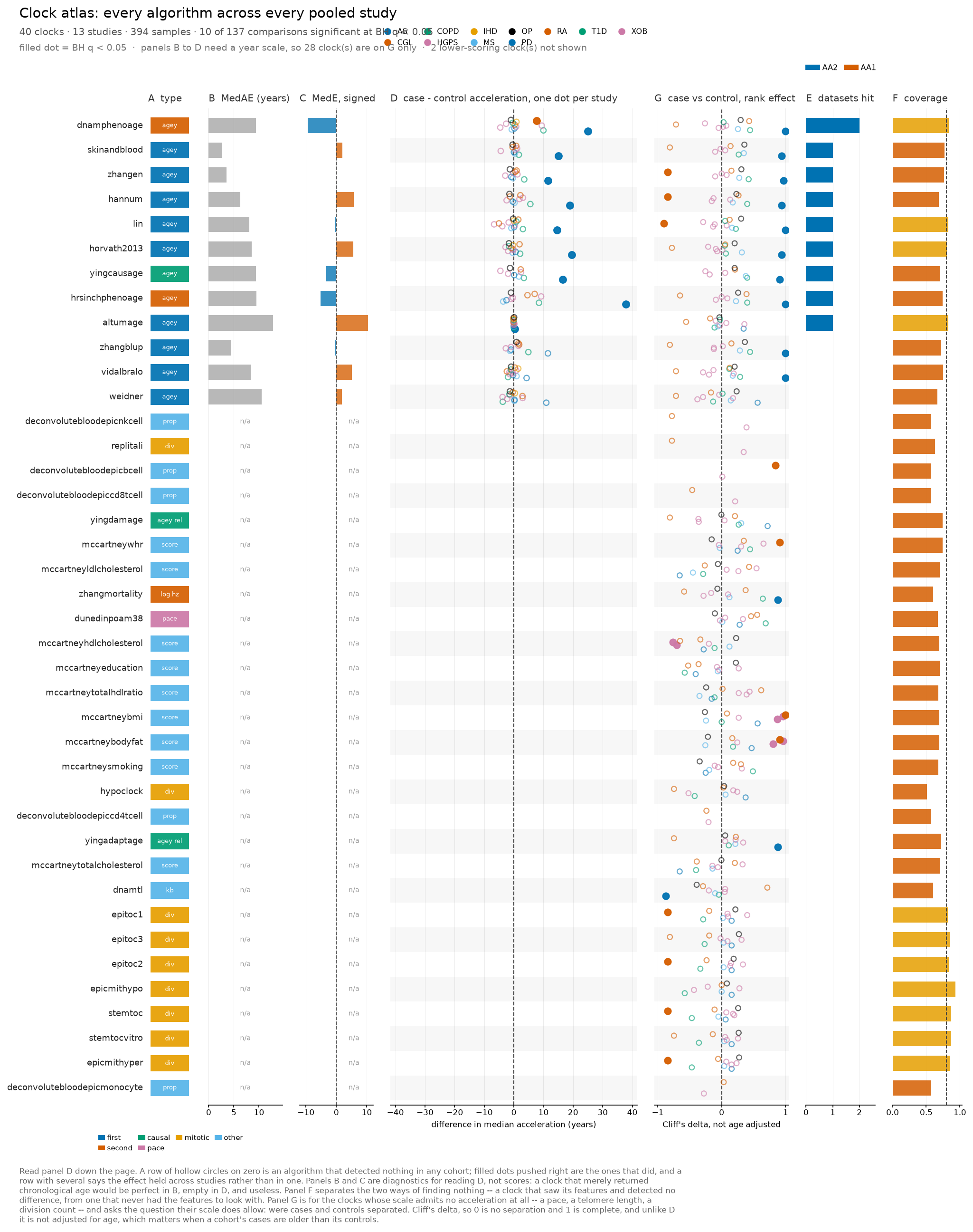
Read panel D down the page. A row of hollow circles on zero is an algorithm that detected nothing in any cohort; filled dots pushed right are the ones that did, and a row with several says the effect held across studies rather than in one. Panels B and C are diagnostics for reading D, not scores: a clock that merely returned chronological age would be perfect in B, empty in D, and useless. Panel F separates the two ways of finding nothing – a clock that saw its features and detected no difference, from one that never had the features to look with. Panel G is for the clocks whose scale admits no acceleration at all – a pace, a telomere length, a division count – and asks the question their scale does allow: were cases and controls separated. Cliff’s delta, so 0 is no separation and 1 is complete, and unlike D it is not adjusted for age, which matters when a cohort’s cases are older than its controls.
plot.clock_atlas() in Python.
Is the clock calibrated
Before any biology: does the prediction track chronological age, and where does it drift.
Predicted against chronological age
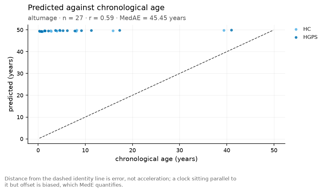
Distance from the dashed identity line is error, not acceleration; a clock sitting parallel to it but offset is biased, which MedE quantifies.
plot.ba_vs_ca() in Python.
Agreement across the age range
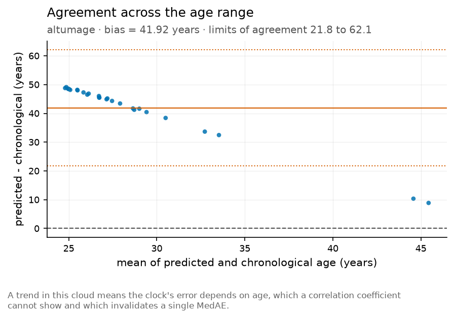
A trend in this cloud means the clock’s error depends on age, which a correlation coefficient cannot show and which invalidates a single MedAE.
plot.bland_altman() in Python.
Residual against chronological age
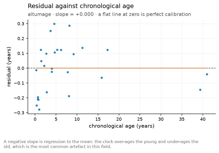
A negative slope is regression to the mean: the clock over-ages the young and under-ages the old, which is the most common artefact in this field.
plot.calibration() in Python.
Age acceleration
The residual after age is removed, by group and across studies.
Acceleration group
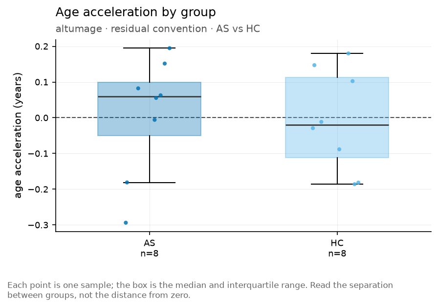
plot.acceleration_group() in Python.
Distribution of age acceleration
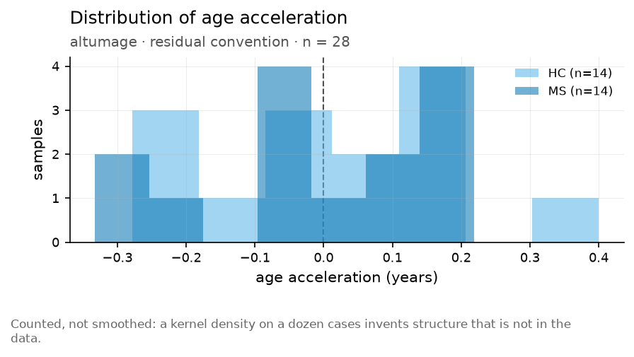
Counted, not smoothed: a kernel density on a dozen cases invents structure that is not in the data.
plot.acceleration_density() in Python.
Age acceleration across clocks and samples
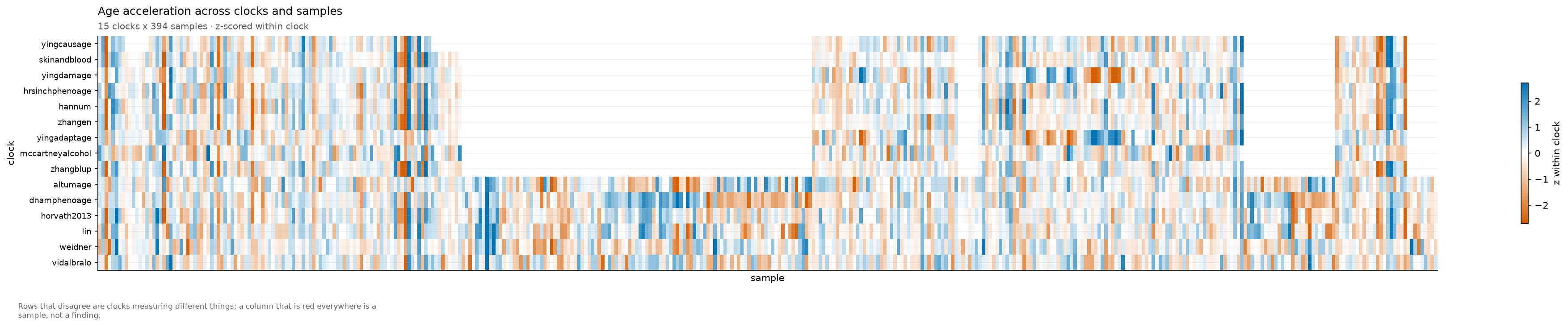
Rows that disagree are clocks measuring different things; a column that is red everywhere is a sample, not a finding.
plot.acceleration_heatmap() in Python.
Effect of condition on age acceleration
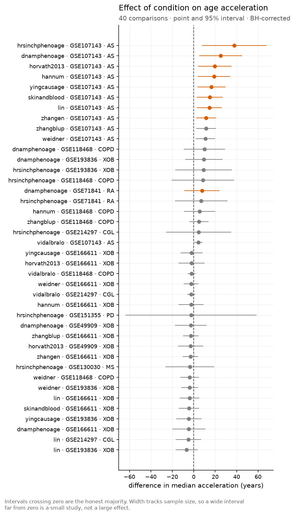
Intervals crossing zero are the honest majority. Width tracks sample size, so a wide interval far from zero is a small study, not a large effect.
plot.forest() in Python.
Outcomes
Whether acceleration predicts anything that happens to a person.
Survival by age acceleration
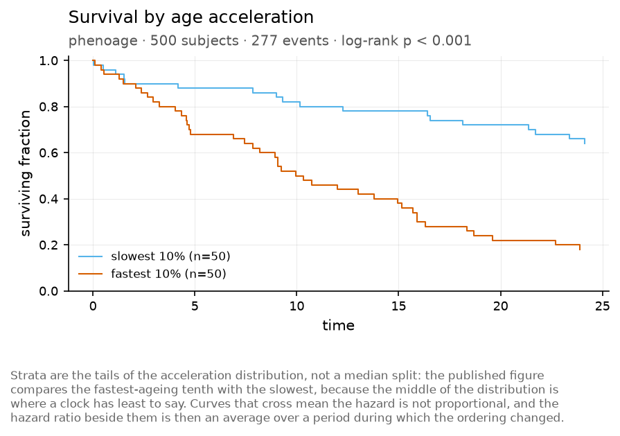
Strata are the tails of the acceleration distribution, not a median split: the published figure compares the fastest-ageing tenth with the slowest, because the middle of the distribution is where a clock has least to say. Curves that cross mean the hazard is not proportional, and the hazard ratio beside them is then an average over a period during which the ordering changed.
plot.kaplan_meier() in Python.
Association with age acceleration
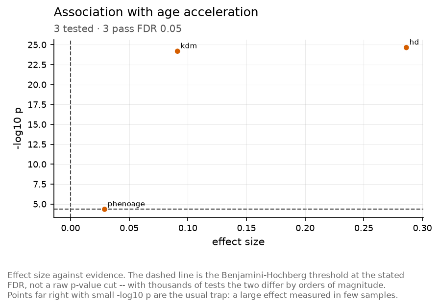
Effect size against evidence. The dashed line is the Benjamini-Hochberg threshold at the stated FDR, not a raw p-value cut – with thousands of tests the two differ by orders of magnitude. Points far right with small -log10 p are the usual trap: a large effect measured in few samples.
plot.volcano() in Python.
How the clocks relate
Twenty clocks are not twenty measurements. These show how much they share – of their features, and of their answers.
Agreement between clocks
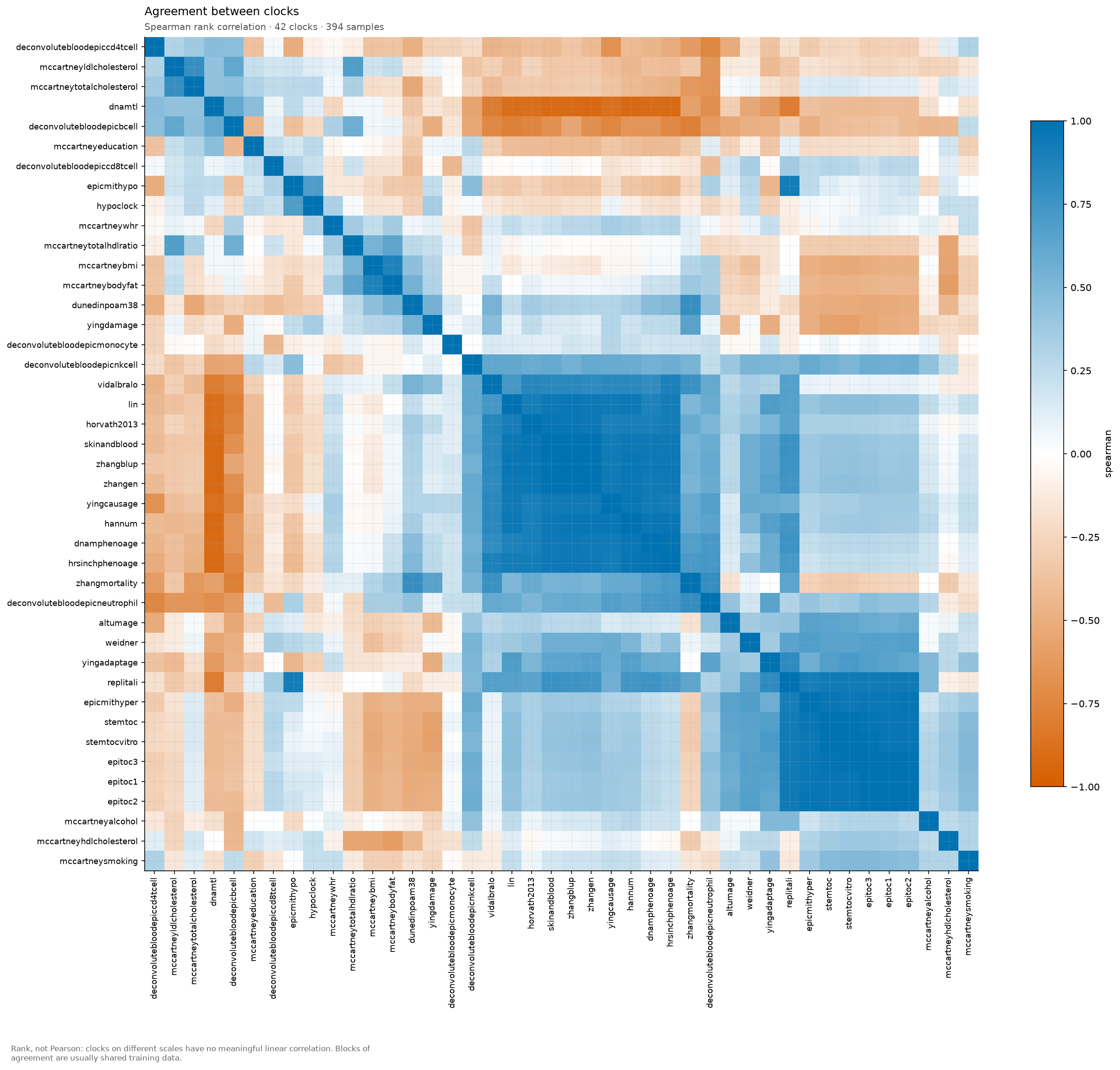
Rank, not Pearson: clocks on different scales have no meaningful linear correlation. Blocks of agreement are usually shared training data.
plot.clock_corr() in Python.
Feature sharing between clocks
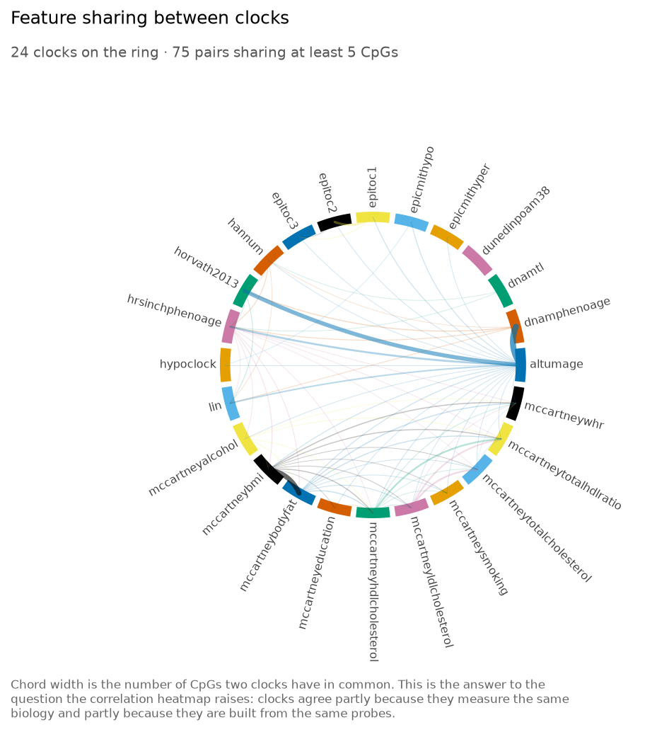
Chord width is the number of CpGs two clocks have in common. This is the answer to the question the correlation heatmap raises: clocks agree partly because they measure the same biology and partly because they are built from the same probes.
plot.clock_chord() in Python.
Multi-clock profile
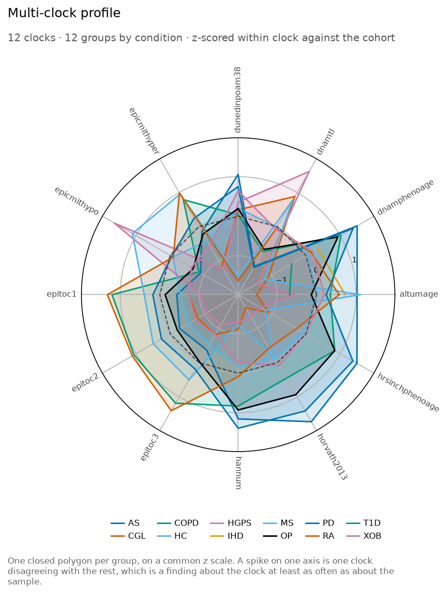
One closed polygon per group, on a common z scale. A spike on one axis is one clock disagreeing with the rest, which is a finding about the clock at least as often as about the sample.
plot.clock_radar() in Python.
Samples in clock space
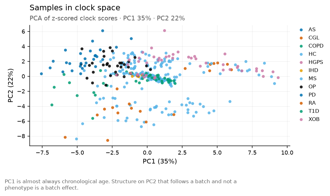
PC1 is almost always chronological age. Structure on PC2 that follows a batch and not a phenotype is a batch effect.
plot.clock_pca() in Python.
Benchmarking
AA1 and AA2 against the ComputAgeBench conditions, and the error-versus-bias tradeoff that decides the ranking.
Datasets detected per clock
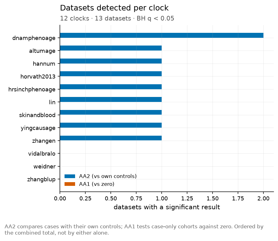
AA2 compares cases with their own controls; AA1 tests case-only cohorts against zero. Ordered by the combined total, not by either alone.
plot.benchmark_bars() in Python.
Error against bias on healthy controls
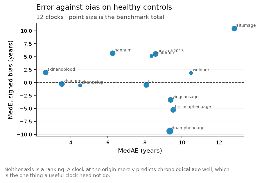
Neither axis is a ranking. A clock at the origin merely predicts chronological age well, which is the one thing a useful clock need not do.
plot.benchmark_error_bias() in Python.
Effect size per clock and dataset
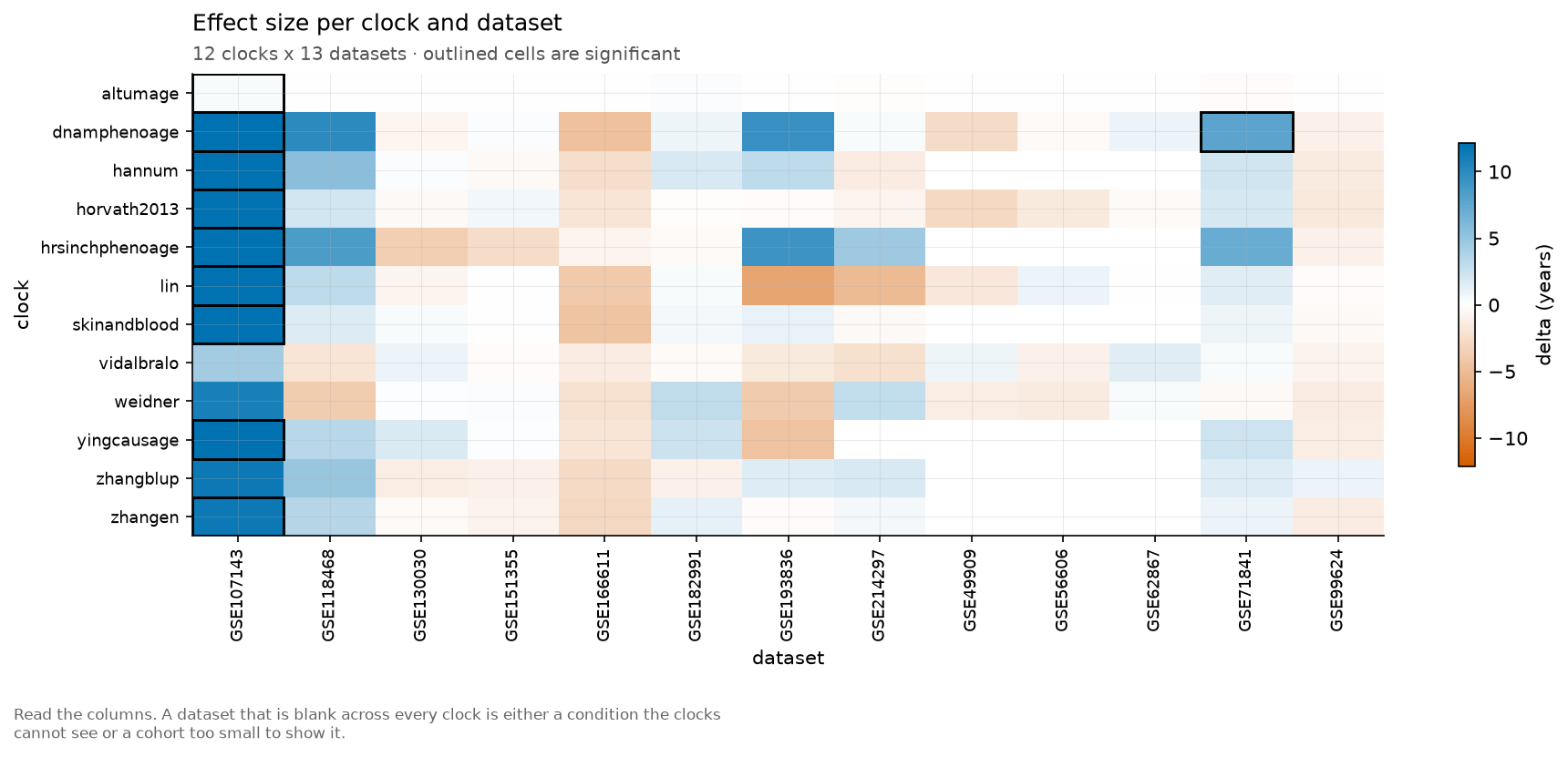
Read the columns. A dataset that is blank across every clock is either a condition the clocks cannot see or a cohort too small to show it.
plot.benchmark_heatmap() in Python.
Data quality
Drawn before the results, because a coverage problem invalidates everything after it.
Feature coverage per clock
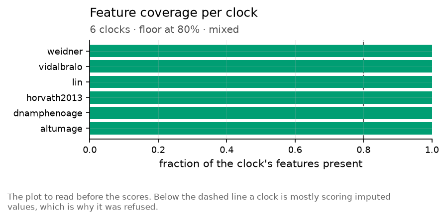
The plot to read before the scores. Below the dashed line a clock is mostly scoring imputed values, which is why it was refused.
plot.coverage_bar() in Python.
Missing values per sample
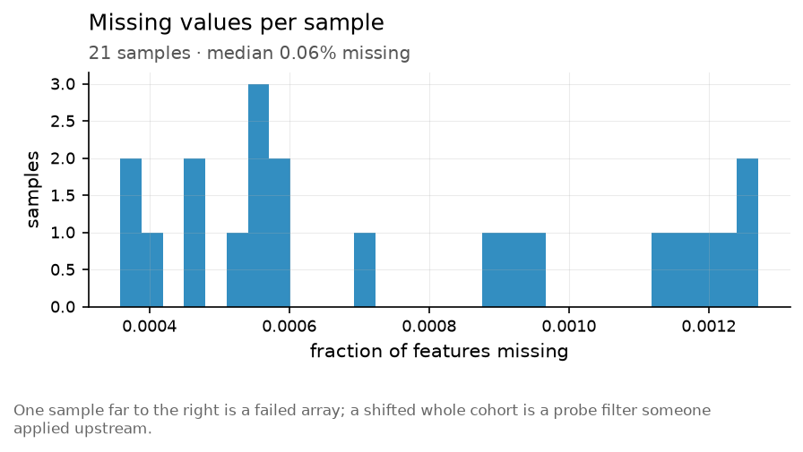
One sample far to the right is a failed array; a shifted whole cohort is a probe filter someone applied upstream.
plot.missingness() in Python.
Beta value distribution per sample
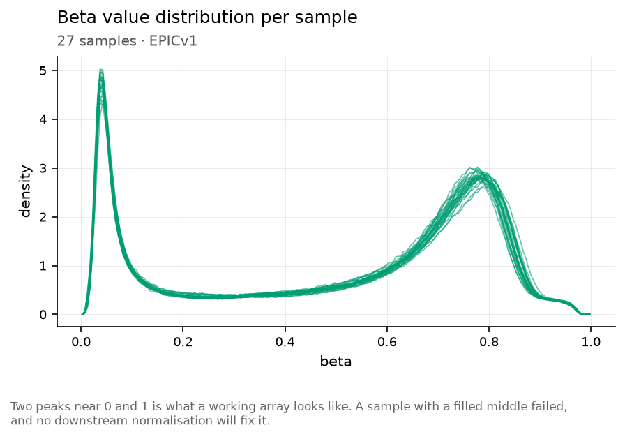
Two peaks near 0 and 1 is what a working array looks like. A sample with a filled middle failed, and no downstream normalisation will fix it.
plot.beta_density() in Python.
Platform
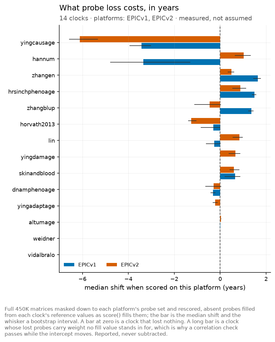
plot.platform() in Python.
Study
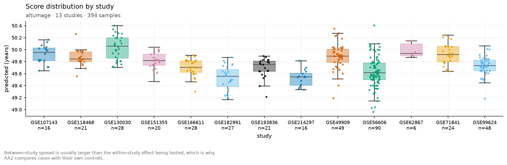
plot.study() in Python.
Other
Figures not yet placed in a section above.
Does the difference hold up across clocks?
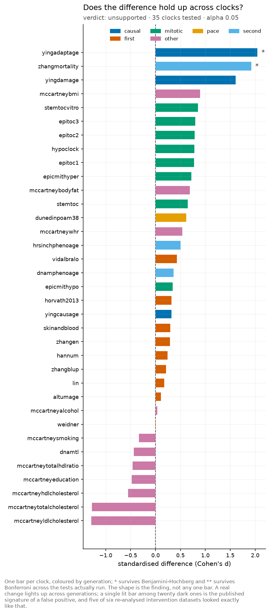
One bar per clock, coloured by generation; * survives Benjamini-Hochberg and ** survives Bonferroni across the tests actually run. The shape is the finding, not any one bar. A real change lights up across generations; a single lit bar among twenty dark ones is the published signature of a false positive, and five of six re-analysed intervention datasets looked exactly like that.
plot.consensus_plot() in Python.
What probe loss costs, in years
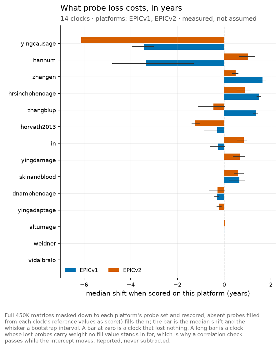
Full 450K matrices masked down to each platform’s probe set and rescored, absent probes filled from each clock’s reference values as score() fills them; the bar is the median shift and the whisker a bootstrap interval. A bar at zero is a clock that lost nothing. A long bar is a clock whose lost probes carry weight no fill value stands in for, which is why a correlation check passes while the intercept moves. Reported, never subtracted.
plot.platform_bias() in Python.
How much of each score is the assay
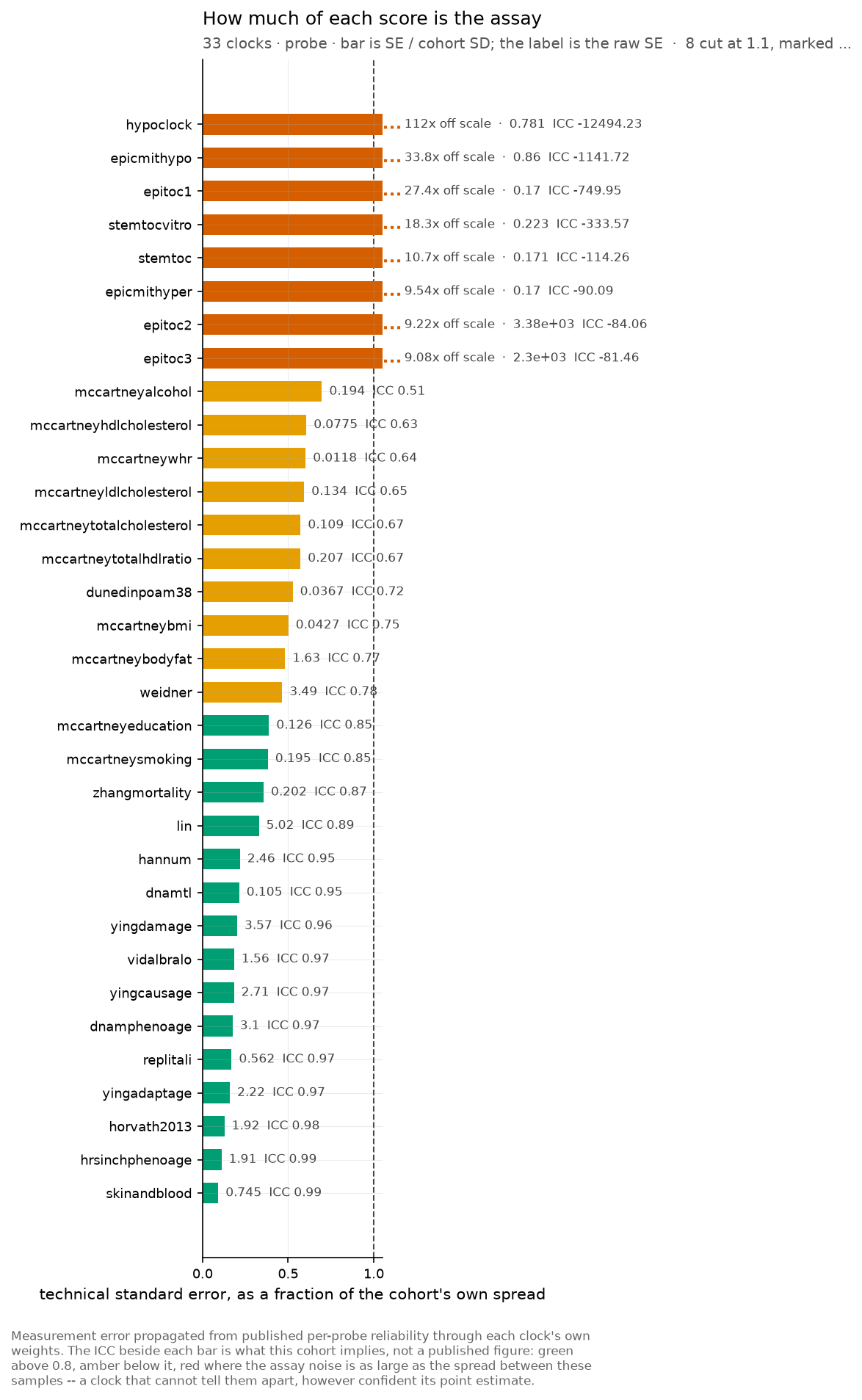
Measurement error propagated from published per-probe reliability through each clock’s own weights. The ICC beside each bar is what this cohort implies, not a published figure: green above 0.8, amber below it, red where the assay noise is as large as the spread between these samples – a clock that cannot tell them apart, however confident its point estimate.
plot.reliability_forest() in Python.
Scores with the uncertainty they carry
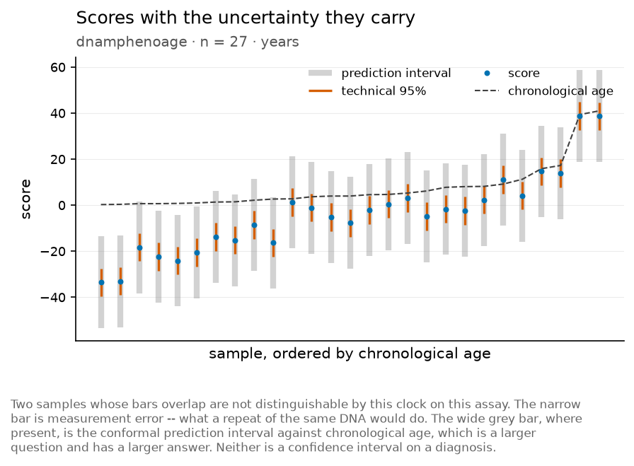
Two samples whose bars overlap are not distinguishable by this clock on this assay. The narrow bar is measurement error – what a repeat of the same DNA would do. The wide grey bar, where present, is the conformal prediction interval against chronological age, which is a larger question and has a larger answer. Neither is a confidence interval on a diagnosis.
plot.score_interval() in Python.
In total
26 figures. Every one is also written per dataset under test/output_figures/<group>/<dataset>/ when the full corpus run is executed; the gallery keeps one representative of each type so a reader does not have to fetch 586 MB to see them.