About cyRAVEN

cyRAVEN turns a folder of FCS files into population frequencies, marker expression, a UMAP and group statistics. This page explains what happens to the data at each stage, and why it is done that way.

New to flow cytometry? Read About flow cytometry first. Want to run something now? Go to Get started.

Why per-sample gates

Manual gating varies between operators. When 38 operators gated the same files, the median expanded uncertainty was 3.6%, and experience made no significant difference (Grant and others, 2021, PDA J Pharm Sci Technol 75:33). Across 320 clinical samples analysed by six technologists on three harmonised cytometers, the remaining spread followed the operator more than the instrument (Mead and others, 2026, Cytometry B, doi:10.1002/cyto.b.70048).

Copying one set of gate coordinates to every sample does not solve this. Staining intensity differs between samples, so a fixed cut is right for some and wrong for others, and the error then follows staining intensity. cyRAVEN places each cut inside its own sample and reports how precisely that cut is determined.

Statistics follow one rule: the sample is the unit, not the cell. A tube run for longer gives more events but no more information about the study, so every test first reduces each sample to one value. Several samples from one donor are not independent either; --paired-column and --condition-column pair them. Anything that cannot be reduced to one value per sample is reported as an effect size without a p-value.

Two ways to use it

	Declared (default)	Explore (`--explore`)
You supply	A list of populations and their marker rules	Only the FCS files
You get	Named populations, with uncertainty and statistics	Numbered clusters over every usable channel
It can find	Only what you listed	Populations nobody listed
Cells used	The CD45+ parent gate	Every event, after its own debris and dead-cell screen

Explore writes to <outdir>/explore/ and changes nothing else, so adding it to a run is safe. --explore-only needs no population list at all. The two halves share nothing unless you add --maybe-learn; see Explore mode.

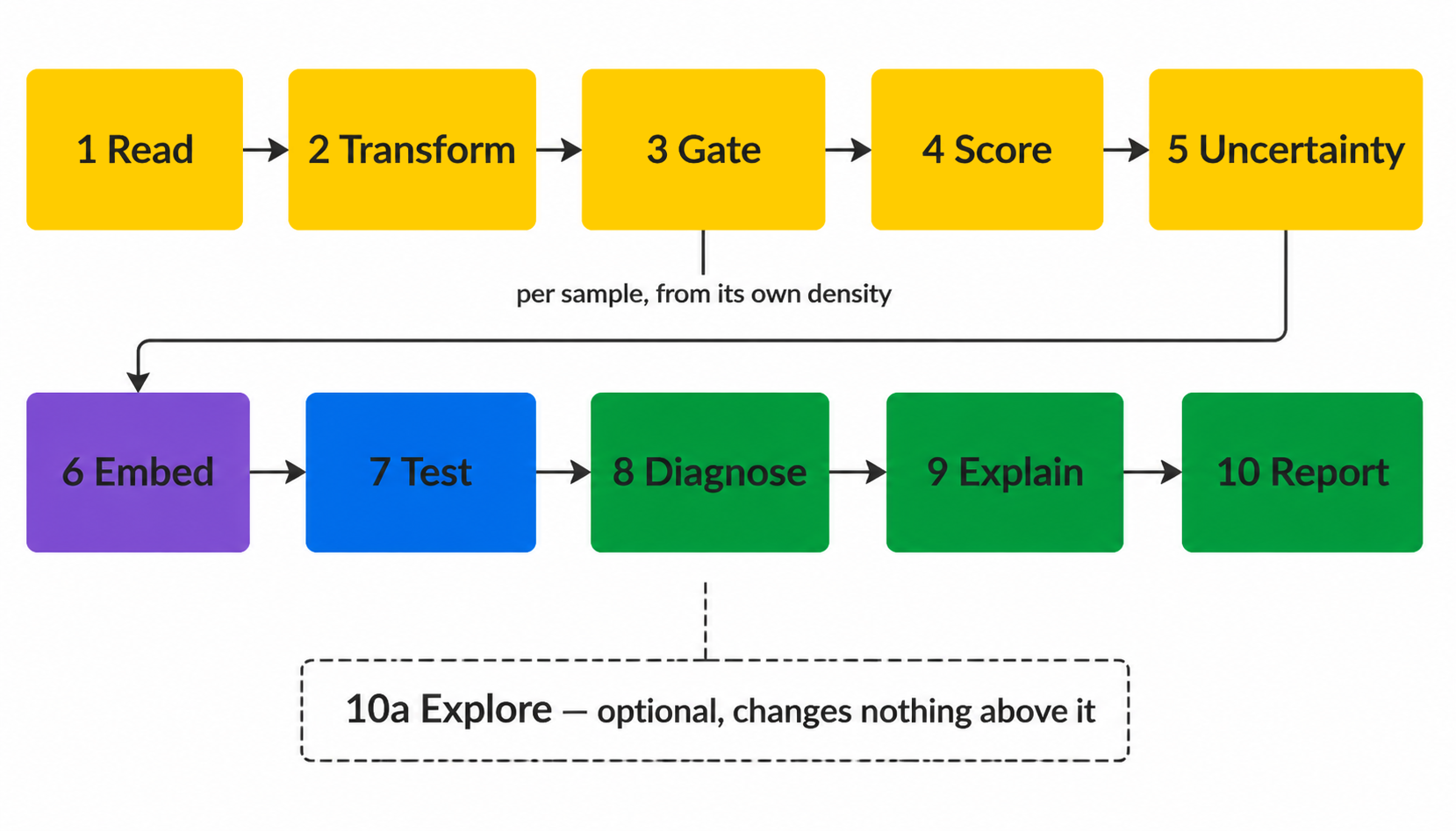
How it works: the ten stages

One call to run_cyraven() runs every stage. Each stage is also an exported function, so you can run or replace a single step.

Stage	In plain words	Function
1 Read	Open each file and work out which channel is which marker	`read_fcs_resolved()`
2 Transform	Put intensities on an arcsinh scale, which spreads the dim end and compresses the bright end	`derive_cofactor()`
3 Gate	In each sample, cut each marker at the lowest point between its negative and positive peaks	`density_valley()`, `resolve_threshold()`
4 Score	Count the cells that meet each population’s rule from your YAML	`score_populations()`
5 Uncertainty	Re-derive every cut on resampled events to see how far it moves	`threshold_uncertainty()`
6 Embed	Build a UMAP with about the same number of cells from each sample	`run_umap()`
7 Test	Compare groups with one value per sample	`stats_group_comparison()`
8 Diagnose	Check whether the gates and populations held up	`stats_threshold_drift()`, `cluster_gate_agreement()`
9 Explain	Describe an unexplained cluster as a gating strategy	`explain_cluster()`
10 Report	Write tables, figures, the run manifest and `report.html`	`write_run_manifest()`

The sections below give the detail for each stage.

The ten pipeline stages in order, with explore mode attached as an optional branch

1 Read

read_fcs_resolved() resolves channels to marker symbols from $PnS with fallback to $PnN, and applies the acquisition spillover matrix where the file carries one. Spectral instruments write unmixed data with no matrix, so maybe_compensate() detects and reports rather than assuming; applying compensation twice is as damaging as omitting it.

2 Transform

set.seed(42)
mk <- c("CD3", "CD4", "CD8", "CD19")
ex <- matrix(abs(rnorm(20000 * 4, 0, 250)),
             ncol = 4,
             dimnames = list(NULL, mk))
cf <- derive_cofactor(
  ex, setNames(1:4, colnames(ex)))
round(as.numeric(cf), 1)

#> [1] 157.2

The arcsinh cofactor governs the width of the quasi-linear region near zero. The conventional value of 5 derives from mass cytometry and over-expands the background band on spectrally unmixed fluorescence data. Each marker is bisected until the interquartile range of its background distribution reaches a target, and the panel adopts the median. derive_cofactor_pooled() estimates across samples so that a single weakly stained file does not set the scale on which every threshold in the run is computed.

3 Gate

# a bimodal marker
x <- c(rnorm(8000, 0, 0.4),
       rnorm(2000, 4, 0.5))
round(density_valley(x), 2)

#> [1] 1.52

Thresholds are placed at the density minimum within each sample. density_valley() returns NA for unimodal distributions, after which resolve_threshold() uses a declared control if there is one, otherwise a tail gate above the dominant mode, and only then a flagged quantile. Derivation is recorded per threshold in thresholds_used.csv.

Per-sample thresholding accommodates staining variation but permits the definition of a population to differ between groups, which stats_threshold_drift() exists to detect.

4 Score

spec <- default_population_spec()
str(spec[["CD3 pos CD4 pos"]])

#> List of 2
#>  $ CD3: chr "above"
#>  $ CD4: chr "above"

Populations are evaluated as Boolean conjunctions of marker directions read from YAML. Editing the specification changes the analysis without modifying R code.

5 Quantify the uncertainty

u <- threshold_uncertainty(
  x_parent, source = "valley", B = 100)
c(u$u_sampling, u$u_method, u$u_combined)

Each cut is re-derived from resamples of its own events, and again across the settings that placed it. The two spreads combine in quadrature and propagate to every population reading that marker, alongside the CD45 parent term, which enters all of them because it fixes the denominator.

The reported threshold is unchanged: the perturbation runs on copies. Every entry point saves and restores .Random.seed, so the cell selection in the next stage draws from the same stream position whether this runs or not.

6 Embed

emb <- run_umap(mat, n_neighbors = 30,
                min_dist = 0.3, seed = 42)

select_umap_features() excludes scatter, viability, time and the height and width duplicates of area channels; retaining these was the principal cause of uninformative embeddings in the precursor implementation. plan_subsample() draws equal cell numbers per sample so that acquisition depth does not determine the manifold.

ret_model = TRUE retains the model for projection of later batches through project_umap(), which holds coordinates fixed between runs. Model retention alters the embedding; see ?run_umap.

7 Test

ids <- sprintf("S%02d", 1:12)
freq <- data.frame(
  sample_id = rep(ids, each = 2),
  population = rep(c("CD4 T cells",
                     "B cells"), 12),
  pct_of_cd45_pos = c(rbind(
    rnorm(12, 25, 4), rnorm(12, 10, 2))),
  is_control = FALSE, qc_status = "pass")
grp <- setNames(
  rep(c("HC", "Patient"), each = 6),
  ids)

res <- stats_group_comparison(
  freq, grp, reference = "HC")
res[, c("population", "comparison_group",
        "n_reference", "cliffs_delta",
        "p_value")]

#>    population comparison_group n_reference
#> 2 CD4 T cells          Patient           6
#> 1     B cells          Patient           6
#>   cliffs_delta   p_value
#> 2       -0.167 0.6991342
#> 1        0.000 1.0000000

stats_marker_state() applies the same treatment to marker expression within a population, testing median intensity and percent positive separately because a shift confined to a subset moves one and not the other.

8 Diagnose

Six outputs constrain interpretation of the preceding stages: threshold drift, gate and counting uncertainty, phenotype concordance, gate against cluster concordance, learned gate geometry, and conformance against a baseline. The Diagnostics covers each in full.

batch_mixing_report() quantifies batch structure in the embedding against a permutation null and reports Cramér’s V between batch and group. Correction through --correct-batch is refused above a configurable V, where batch and biological effect are not separable.

stats_threshold_drift() tests whether marker thresholds separate by group, which would render an abundance difference partly definitional.

stats_confounding() reports whether a covariate both differs across groups and associates with the outcome within groups, the two conditions jointly defining a confounder.

cluster_gate_agreement() cross-tabulates declared labels against unsupervised clusters, which can reveal a population absent from the specification, or a threshold rejecting events that belong to its population.

run_gate_uncertainty() reports how far each threshold moves under resampling and propagates that to every population reading it, so a difference smaller than its own gate’s movement is identifiable as such.

9 Explain

cluster_gate_agreement() identifies a cluster matching no declared population but cannot characterise it, leaving a cluster index and a cell count.

explain_cluster() inverts the gating stage. Given labelled events it selects the two most discriminating markers, fits a convex polygon in that plane, retains the enclosed events and recurses, producing the topology of a manual gating strategy.

st <- explain_cluster(marker_matrix,
                      cluster_id == 7)
# marker pair and metrics per level
st$summary
# vertices, on the analysis scale (arcsinh or logicle)
st$levels[[1]]$polygon

Convex polygons rather than thresholds: a conjunction of one-dimensional cuts is an axis-aligned rectangle, and an oblique boundary constrained to a rectangle must admit contaminants or exclude genuine events. derive_singlet_band() is a hand-written instance of the same geometry.

Metrics are computed on held-out events with the resubstitution value alongside, since eight free half-planes can memorise a few thousand events. The stage is descriptive: it carries no p-value and scored frequencies are identical whether it runs or not.

--external-labels supplies the labels from elsewhere, a cyCONDOR clustering for instance, and gate_transferability() then refits the strategy with one donor withheld and scores it on that donor. Held-out events come from the same donors and overstate how well a gate travels; the per-donor minimum does not. --export-gates writes the result as Gating-ML 2.0 on the scale it was fitted on, and as a vertex table in the units the FCS file stores.

10 Report

Figures, tables, and write_run_manifest(), which records R version, package versions, git commit and working-tree state, the full invocation, and every input file with size and modification time. The manifest is written before the expensive stages and rewritten at completion, so an interrupted run records status: failed.

10a Explore

--explore runs a second, independent analysis over the single cells of every file (scatter and singlet gates only) and every eligible channel, writing to <outdir>/explore/ and leaving stages 1 to 10 untouched. It has its own quality gate, its own embedding and clustering, and its own self-contained report. --explore-only runs it without stages 2 to 10 at all. See Explore mode.

Why explore mode is built this way

The design record for explore mode: what the supervised and unsupervised halves can lend each other, which of those exchanges are implemented, which are refused, and where that leaves cyRAVEN against the tools it sits beside.

Written because “add unsupervised clustering” is the easy half of the problem. The hard half is deciding what the two halves are allowed to tell each other without losing what made each one useful.

1. The two failure modes

Supervised and unsupervised cytometry analysis fail in opposite directions, and neither can detect its own failure.

Supervised analysis cannot find what it was not told to look for. You declare twelve populations, it scores twelve populations. A thirteenth cell type sits in the data unremarked. Worse, a declared label may cover two distinct phenotypes, and their total can stay flat while one rises and the other falls. That is a real pattern that no amount of testing on the declared table can surface, because the table has one column where the biology has two.

Unsupervised analysis cannot tell you what it found. FlowSOM returns cluster 17. Whether cluster 17 is a B cell subset, a doublet artefact, or the same cells as cluster 4 under a different sampling seed is left to a human squinting at a heatmap. And because the clusters are defined on the data, the number of them that reach significance moves with parameters nobody reports. Measured elsewhere in this project, one cyCONDOR run went from 1 significant cluster to 8 by changing only how many cells were drawn.

Running both and reading them side by side does not fix either. What fixes them is deciding which specific facts may cross between them.

2. The exchange, enumerated

Every transfer that is technically possible between the two halves, with the verdict on each.

2.1 Declared -> explore

What could be lent	Verdict	Why
The transform and its estimated cofactor	Always	A property of the panel derived from the data, not a product of the declaration. An unsupervised tool assumes a transform; cyRAVEN estimates one. Lending it costs nothing and removes an arbitrary constant
Per-sample thresholds	Under `--maybe-learn`	The single largest gain. See section 3
Staining QC verdicts	Under `--maybe-learn`, as a column	Recorded, never used to exclude. See section 4
Batch/group confounding verdict	Under `--maybe-learn`	Without it explore reintroduces the exact failure the declared path refuses. See section 5
Group labels	Always	They come from the sample sheet, not from the analysis. Withholding them would mean explore could not test anything
The parent gate	Never	Explore exists to look outside it. Applying it would make explore a re-clustering of the declared result
The population definitions	Never	That is the thing being checked

2.2 Explore -> declared

What could be lent	Verdict	Why
Populations spanning several clusters	Under `--maybe-learn`, as `spec_gaps.csv`	The finding the declared path structurally cannot make about itself
Clusters no population covers	Under `--maybe-learn`, same file	Names what the specification missed
Cluster-derived population definitions, adopted automatically	Never	Circular. See section 6
Re-gating, re-thresholding, or altering any declared frequency	Never	A run whose numbers were changed by a clustering is no longer the run its manifest describes

The asymmetry is deliberate. Explore may describe the declared analysis. It may never alter it.

3. Per-sample thresholds: the exchange that matters most

A standalone clusterer names a cluster by pooling every cell, computing a median per marker, and putting a colour scale on it. Three things are wrong with that on multi-sample data, and all three are things cyRAVEN has already solved for the declared path:

The pooled median is not a threshold. It is the middle of the distribution, which for a marker where 80% of cells are positive sits inside the positive population.
It ignores staining variation between samples. A bright sample and a dim one are compared against one number, which is precisely the systematic bias that per-sample gating exists to remove.
It produces a colour, not a call. “Reddish for CD19” is not a measurement.

Under --maybe-learn, explore reads thresholds_used.csv and calls each cell against its own sample’s cut. A cluster’s phenotype becomes:

CD19+ HLA-DR+ CD3- CD14-

where every + means this fraction of the cluster’s cells were above the threshold derived in their own sample, recorded in frac_pos.<marker> columns. A marker the cluster is mixed for is omitted rather than called either way, so the phenotype string admits what it does not know.

That is a claim no standalone clusterer can make, and it is not a clever algorithm. It is the reuse of work the declared path already did.

4. Two things explore can do that the declared path cannot

It keeps the samples staining QC excluded. A sample with no resolvable CD45 mode has no usable parent gate, so every declared percentage from it would be a fraction of an arbitrary slice of the scatter plot. The declared path must drop it. Explore does not depend on that gate, so those samples still contribute, and staining_qc_verdict is a column rather than a filter. On the KMT2 cohort analysed in this project that is three donors the declared path had to discard and explore can still describe.

It looks outside the parent gate. Anything the CD45 gate excluded is invisible to the declared analysis by construction. Explore embeds it, which is how a population that fails the parent gate can still be seen.

5. Carrying the confounding verdict

The most likely way explore mode could damage this package is by becoming a p-value generator that ignores everything the declared path established.

explore_cluster_stats.csv therefore carries batch_group_cramers_v and batch_group_verdict as columns of the results table itself, not as a note elsewhere. On a cohort where batch and group are confounded, a q < 0.05 on a cluster means exactly as little as a q < 0.05 on a declared population, and the table says so on the same row.

Explore’s statistics are also donor-level, using the same stats_group_comparison() the declared path uses: one value per sample, Kruskal-Wallis omnibus, Wilcoxon pairwise, Cliff’s delta, Benjamini-Hochberg. Not a reimplementation: the same function, so the two cannot drift apart.

6. Why the draft specification is never adopted automatically

explore_suggested_spec.yaml turns clusters into declarable population definitions. The obvious next step, feeding it straight back into the declared pipeline, is refused, and this is a central design decision in the feature.

cyRAVEN’s argument is that populations are declared before the data are examined, and six diagnostics then try to falsify that declaration. Derive the specification from the same data and the diagnostics become circular:

Phenotype concordance asks whether a population expresses the markers its definition demands. Trivially yes, if the definition was read off those cells.
Gate-cluster concordance compares declared gates against unsupervised clusters. If the gates came from those clusters, it compares a thing to itself.

There is a sharper version. Explore’s clustering is group-blind. It never sees cohort labels, so deriving a definition from cluster phenotypes is a mild form of double-dipping. But explore_cluster_stats.csv does test by group. A user who reads that table, sees which clusters differ, and declares those as populations has selected on the outcome, and every subsequent p-value is invalid.

The defensible uses, ranked:

Workflow	Verdict
Explore on cohort A -> curate -> declared run on cohort B	Clean. The intended loop
Explore -> curate -> declared run on the same cohort, reporting frequencies	Acceptable; state that the spec was data-derived
Explore -> read the group statistics -> declare the clusters that differed	Invalid. Selection on the outcome

Hence: a YAML file whose header says it is a suggestion, requiring a human edit, with no flag anywhere that adopts it.

7. Choices inherited rather than invented

Three decisions were taken from the unsupervised literature because they are better than what a supervised tool would reach for.

Cluster everything, including scatter and viability. No lineage preference. This is what lets the QC gate find debris (leukocyte marker low), dead cells (viability high) and granulocytes, which no antibody in most panels identifies. The cost is real: some clusters split on scatter rather than lineage. --explore-markers overrides it.

Gate on clusters, not events. Cluster coarsely first, then judge whole clusters by their median profile, so no per-event cutoff is invented. The units judged are the SOM nodes rather than the merged clusters, because a merge can join debris to the CD45-dim cells beside it. The debris and dead calls come from 2-means on the per-node medians when nothing better is available, and from per-sample thresholds when it is. Both are recorded in the basis column of explore_qc_clusters.csv.

Refuse a gate that keeps almost nothing. Below --explore-min-retained (default 5%), the gate is ignored and the run flagged: at that point the markers are likelier mis-named than the data bad.

One decision goes the other way. Cells are re-equalised per sample after the gate. cyCONDOR does not do this, and its faceted panels then differ in density for a reason that is group size rather than biology. That trap was documented while running it during this project. Equalising costs cells and buys panels that can honestly be read side by side.

8. Where this leaves cyRAVEN

Compared with FlowSOM, Phenograph, cyCONDOR, diffcyt and CATALYST:

Capability	cyRAVEN	Also in
Per-sample gate derivation	yes	none of them
Uncertainty carried to every frequency	yes	none of them
Detection limits per population	yes	none of them
Donor-level inference by construction	yes	diffcyt; possible but not enforced in cyCONDOR and CATALYST
Refuses batch correction when confounded	yes	none of them
Unsupervised discovery	yes	all of them
Clusters named from per-sample thresholds	yes	none of them
Cluster turned into gate geometry	yes	none of them
Gating-ML 2.0 export	yes	none of them
Empirical-Bayes moderation across clusters	no	diffcyt
Trajectory inference	no	cyCONDOR
Cluster count found from the data	no	Phenograph, and cyCONDOR through it. FlowSOM and CATALYST are given the count

The gap this feature closes is the “unsupervised discovery” row. The row that remains distinctive is clusters named from per-sample thresholds, which requires both halves in one tool and is why bolting FlowSOM onto a supervised pipeline is not the same thing.

What is deliberately not adopted

diffcyt’s empirical-Bayes moderation as the primary test (edgeR, limma-voom, GLMM). It borrows strength across clusters via a shared dispersion prior, which pays off at mass-cytometry marker counts with hundreds of clusters. On a declared panel of a dozen populations there is little to borrow, so the rank tests on one value per donor stay primary. The edgeR form, with diffcyt-DA-edgeR’s defaults applied to each sample’s exclusive-label counts, is available beside them with --edger; limma-voom and the GLMM are not implemented.

A data-determined cluster count. Phenograph and consensus methods choose k from the data. --explore-k is a setting, and explore_provenance.csv says so, because a k chosen from the data is one more thing the significance count depends on.

Trajectory inference. Diffusion maps and pseudotime need a differentiation continuum the design supports. On cross-sectional human cohorts of 10 to 40 samples it produces a picture, not a measurement.

9. The claim worth testing

If there is a methods paper here, the claim is not “cyRAVEN clusters cells”. It is:

Threshold placement uncertainty, derived per sample and propagated to reported frequencies, predicts the between-operator variance that manual gating produces, and that populations whose propagated uncertainty is large are the ones where published cohorts disagree.

That is falsifiable and, as far as this project’s reading goes, untested. It would need the same files gated by several operators, with the propagated uncertainty compared against the observed spread of their results. The inter-laboratory data to do it exists in the literature this package already cites.

The second claim, weaker but easier to support: a refusal rule is a feature. A tool that declines to run batch correction above a measured Cramér’s V between batch and group, and says why, produces fewer results and more defensible ones. That one needs a demonstration rather than a benchmark: a cohort where correction would have produced a clean, wrong answer.