
From nothing to a finished run in four commands, then how to describe your own cohort.
Two habits save the most time:
-
Run
--checkfirst. It reads only the file headers and stops, so a misspelled marker costs seconds instead of a whole run. -
Open
gating_qc.pngbefore using a number. It draws each cut on the data it came from. A cut on the side of a peak shows there, and in no table.
Setup
You need Docker.
The image fixes R 4.4.3, a dated CRAN snapshot and Bioconductor 3.20. Gates sit at density minima and the UMAP is stochastic, so other package versions can move both slightly.
To build the image yourself instead, for example after changing the source:
git clone \
  https://github.com/bhagesh-h/cyRAVEN
cd cyRAVEN
docker build -t cyraven:1.0.0 \
  -f inst/scripts/Dockerfile .
The first build compiles every R dependency and takes tens of minutes.
To install without Docker, see the README.
Quick start
1. Write the demo data. 35 FCS files from five transplant recipients, a sample sheet and a config. They ship inside the image, so nothing is downloaded.
2. Check the inputs. It should end with
no problems found.
docker run --rm \
  -v "$PWD/demo:/data:ro" \
  -v "$PWD/results:/results" \
  cyraven:1.0.0 \
  --dir /data/fcs \
  --samples /data/samples.csv \
  --config /data/panel.yaml \
  --group-column cohort \
  --reference-group "GvHD grade 1" \
  --outdir /results \
  --check
3. Run it. A few minutes.
docker run --rm \
  -v "$PWD/demo:/data:ro" \
  -v "$PWD/results:/results" \
  cyraven:1.0.0 \
  --dir /data/fcs \
  --samples /data/samples.csv \
  --config /data/panel.yaml \
  --group-column cohort \
  --reference-group "GvHD grade 1" \
  --outdir /results
4. Open results/report.html. Every
figure and table is in that one file, in the order to read them.
Paths in the flags are paths inside the container, and
--outdir must be in a mounted folder or the results vanish
when the container exits. On Windows, run these in Git Bash or WSL with
MSYS_NO_PATHCONV=1 in front of each command. In PowerShell,
end each continued line with a backtick instead of \, and
write ${PWD} for $PWD.
About this cohort: both groups are transplant recipients. The comparison is GvHD grade 1 against grade 3, not disease against health. The groups are small, one patient against four.
Your own data
Two files besides the FCS folder:
| File | Holds |
|---|---|
Sample sheet, samples.csv
|
One row per FCS file: sample, patient, group, timepoint, batch |
Config, analysis.yaml
|
One entry per population: its marker rule,
e.g. CD3: above
|
Start both from a template:
docker run --rm -v "$PWD/data:/data" \
  cyraven:1.0.0 \
  --dir /data/fcs --recursive \
--write-samples /data/samples.csvFill in the sheet and edit the populations: section of
the config. Run with --check until it reports no problems,
then run without it. The full sequence is in A first run on a new cohort. The
rest of this page explains each file and every option.
Inputs: the sample sheet and the config
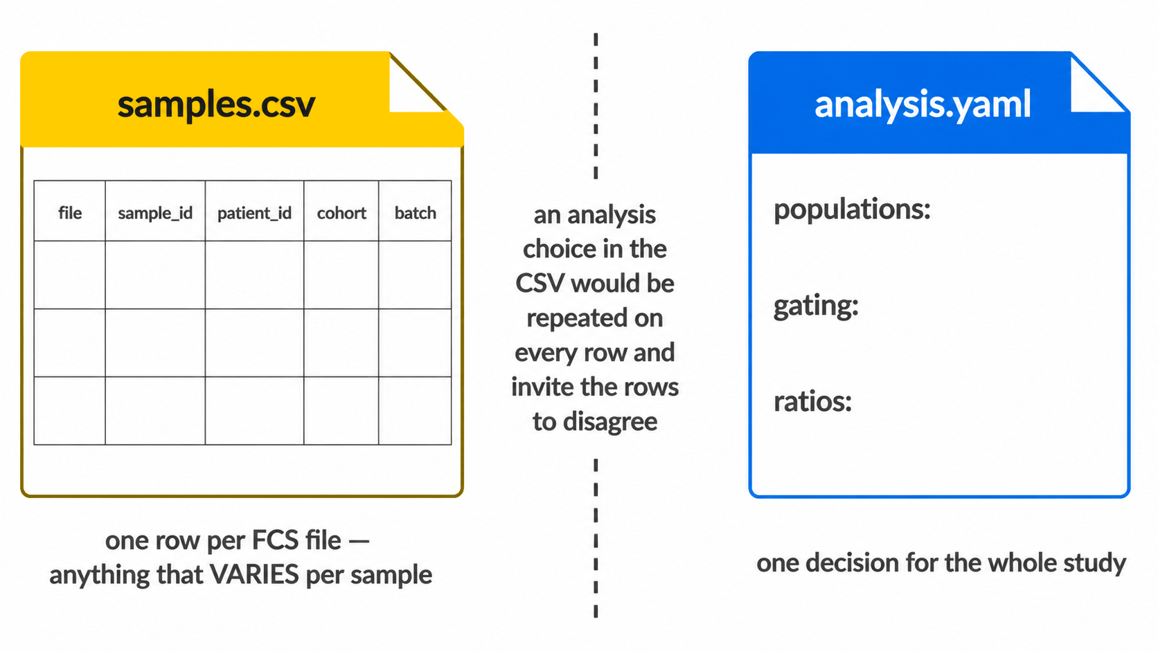
Anything that varies per sample belongs in the sheet; anything that is one decision for the whole study belongs in the config. A study-wide choice put in the sheet would repeat on every row, and the rows could then disagree about it.
From R, the two templates are
write_config_template("analysis.yaml") and
system.file("examples", "samples_template.csv", package = "cyRAVEN").
1. Build the sheet
Do not write it from scratch. Generate one covering every file in the input directory, then fill in the columns only you know:
docker run --rm \
  -v "$PWD/data:/data" \
  cyraven:1.0.0 \
  --dir /data/fcs \
  --write-samples /data/samples.csv
Every acquisition gets a row with its filename and a derived identifier, so the sheet accounts for every file before you touch it. A file the sheet does not cover is a fatal error rather than a guess: inferring which patient a file belongs to from plate order silently mislabels patients, and a mislabelled patient is not visible in any output.
Then check it, which costs seconds because it reads FCS headers and not events:
docker run --rm \
  -v "$PWD/data:/data:ro" \
  -v "$PWD/results:/results" \
  cyraven:1.0.0 \
  --dir /data/fcs \
  --samples /data/samples.csv \
  --config /data/analysis.yaml \
  --outdir /results \
  --check
--check reports the markers it resolved from the files,
the specification entries matching none of them, whether the sheet
covers every file, the levels of the group column and their sizes, the
number of batches, and the study variables available. It analyses
nothing and writes nothing. Run it after every edit to the sheet; a
marker-name mismatch found here costs a second, and found during a run
costs however long the run had been going.
2. Columns of the sheet
Only file is required. Everything else is optional, and
a column that is absent disables what depends on it.
2.1 Which file this is
| Column | Meaning |
|---|---|
file |
The FCS filename. Matched on basename, so a file moved between subdirectories still matches. Required. |
sample_id |
The identifier used in every output. Derived from the filename when absent. |
well |
Plate well, used as the identifier when sample_id is
absent. |
patient_id |
The subject. Several rows may share one, which is what makes repeat acquisitions and longitudinal designs work. |
panel |
Forces a panel assignment. Panels are fingerprinted from the channels otherwise. |
timepoint |
Visit or draw. |
is_control |
TRUE for a control tube. Controls are read and used as
references but excluded from between-group tests. Setting it
FALSE is not the same as leaving it out: FALSE
asserts that the file is a biological sample, and the assertion matters.
See below. |
Say FALSE rather than saying nothing
An absent is_control column means “unknown”, not “no
controls here”. The distinction has teeth.
A control tube supplies the reference distribution for markers that resolve no density minimum, and the cut is then the 99.5th percentile of the control. That is correct when the reference really is unstained. When it is a stained biological sample, the cut lands at the top of a real distribution and the population beneath it all but disappears.
Up to version 1.0.0 a sample that failed staining QC could be promoted to that reference on a sheet that named no controls, on the reasoning that an unlabelled tube might be one. On a cohort of twelve patient samples with no controls at all, that put T cells at 0.034% of CD45+ where the correct figure was over a hundred times higher, with no error and no warning.
cyRAVEN now believes a control only when the sheet declares one, and says so in the log when it declines to promote a sample. Two habits follow from that:
- Write
is_controlon every row,FALSEfor samples andTRUEfor controls.--write-samplesdoes this for you. - If most rows of
thresholds_used.csvreadcontrol_q995in thesourcecolumn, check which sample supplied the reference before reading any frequency. |fmo_for| Comma-separated markers this file is the fluorescence-minus-one control for. | |control_group| Confines a control to the samples sharing its value, since a reagent lot changes between batches. |
2.2 Whose it is
These describe the subject, so they repeat on every row of that subject.
patient_id, date_of_birth,
sex, age_years, height_cm,
weight_kg, infection_focus,
cohort, wbc_per_ul.
They are recognised by their canonical name and by the spellings
common in clinical exports, in English and German, so a sheet headed
Geschlecht or Patient ID resolves without
being translated first. Values are coerced the same way whichever route
supplies them: decimal commas, dates whose day and month order is
resolved from the column as a whole, and sex and clinical vocabulary
translated through a dictionary that passes unknown values through and
reports them rather than mangling them. Extend the dictionary under
metadata: in the YAML.
Age is derived from date_of_birth when it is missing,
against --reference-date. Set that to a fixed study date,
or ages change as the calendar moves and two runs of the same data
disagree.
A subject’s rows must agree. This is the one hazard
the one-file shape introduces that separate tables did not have: with a
row per file, a patient with three acquisitions carries three copies of
their sex. If two disagree, the run stops and names every conflict as
subject / column: value vs value. There is no defensible
way to pick one, and picking silently is how a cohort acquires a patient
who is both male and female depending on which tube you look at.
A blank is not a disagreement. It is filled from the rows that have a value.
2.3 What was measured externally
Any column named count.<Population> is read as an
externally measured absolute count for that population, from bead-based
or volumetric counting.
file,sample_id,count.Monocytes
HC-01.fcs,HC-01,420
A frequency is a proportion of a parent gate, so it moves whenever
any other population moves. An absolute concentration does not, which is
why these are worth carrying when the laboratory measured them. Blanks
are skipped rather than read as zero. Units are cells/uL
unless samples: count_unit: cells/mL says otherwise, in
which case values are divided by 1000.
3. The config
populations: is the only required section. Everything
else takes a documented default when omitted, and the default in force
is stated in the run log.
Populations, functional blocks and ratios are covered in the the gating specification; thresholds, colours and metadata dictionaries in the Running cyRAVEN. One section belongs here, because it is about the sheet:
Naming the roles here means the two files specify the run on their own, with no further flags. A flag still wins where both are given: the config is the study’s standing choice, the flag is this run’s.
4. The older three-file format
--sample-map, --patient-table and
--absolute-counts still work exactly as before and are not
deprecated. Runs made with them remain reproducible.
They cannot be combined with --samples. The sheet
carries the same facts, and two sources of truth for one fact is what
this format removes.
The sheet is a different way to supply the same facts, not a different analysis. The reader splits it into the same three structures the pipeline always consumed and applies the same coercions by calling the same code. A test runs one study both ways and compares every output.
Which to use:
| Situation | Use |
|---|---|
| A new study | The sheet. One key, one file, no joins. |
| An existing pipeline built on the three files | Leave it. Nothing has changed. |
| Counts exported by the counting instrument as its own sheet |
--absolute-counts reads that file’s own layout; see the
Every output file. Fold it
into the sheet only if transcribing it is easy. |
5. Worked example
The full sequence for a new cohort, with the two edits that come between the commands, is in A first run on a new cohort under Commands.
6. When it goes wrong
A run that fails writes report.html anyway, with the
error, the stage it reached, the log leading up to it, what the error
means for the data, and the next action. Everything produced before the
failure is embedded below the diagnosis, because that partial output is
usually where the evidence is.
The errors this format can raise, and what each means:
| Message | Cause |
|---|---|
these input files are not in the sample sheet |
The sheet has no row for a file. Add rows, or regenerate with
--write-samples. |
conflicting values for the same subject |
Two rows of one subject disagree. The message names each conflict. |
duplicate file entries |
Two rows name the same file. |
must contain a 'file' column |
The one required column is missing. |
--samples supersedes ... |
The sheet was combined with a flag it replaces. |
Every population reported UNAVAILABLE, or an empty
frequency table, is almost usually a marker name that does not match
$PnS exactly. --check lists every marker the
files carry and names the specification entries matching none of
them.
The gating specification
Cell identification in cyRAVEN proceeds in three stages: exclusion of non-cellular and non-viable events, placement of per-sample marker thresholds, and evaluation of a declarative population specification against those thresholds. This article documents each stage and the parameters governing it.
1. Hierarchy
Four sequential gates precede any marker evaluation. Each is derived from the data rather than transferred between samples.
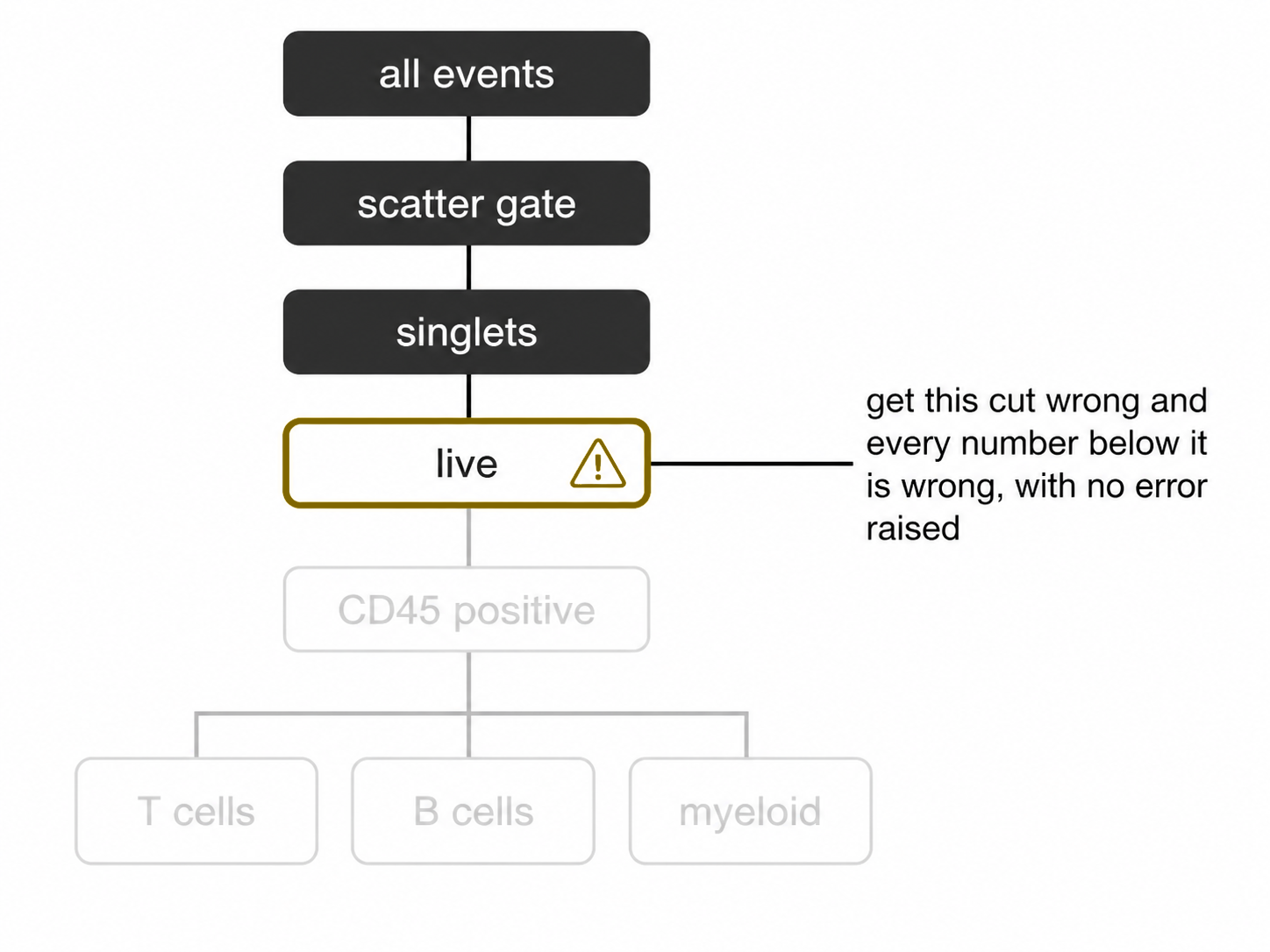
1.1 Scatter. The lower forward-scatter bound is placed at the deepest minimum of the log10 FSC-A density. Sub-cellular debris forms a distinct low-scatter mode separated from intact cells; the minimum between them is the boundary.
1.2 Singlets. Coincident events traverse the
interrogation point over a longer interval than single cells, producing
a pulse whose area is inflated relative to its height, so they have a
low FSC-H:FSC-A ratio. Events are retained above median − k·MAD
of that ratio, computed inside the scatter gate, with k set by
--singlet-mad-k (default 3). The gate is one-sided: a high
ratio is no sign of a doublet.
1.3 Viability. Amine-reactive viability dyes
penetrate only cells whose membrane integrity has been lost. Dead cells
are excluded at the density minimum of the dye channel above the live
cells’ mode, or at a tail gate above that mode where there is none.
Panels without a viability marker skip this gate, and the omission is
logged. Each sample’s live share of single cells is reported in
staining_qc.csv; --min-live-pct fails samples
below the assay’s minimum. Where the dye also has a minimum below its
dominant mode, the share below it is reported too
(pct_live_if_dominant_dead): the live share if the dominant
mode is the dead cells, which the gate cannot tell from a second live
mode near zero.
1.4 CD45. Leukocytes are selected on CD45, which is expressed across haematopoietic lineages and absent from erythrocytes and platelets. Where CD45 is not in the panel, all viable events become the parent and a warning is issued, since percent-of-leukocytes and percent-of-viable are not interchangeable denominators.
All subsequent population frequencies are expressed as a percentage of the CD45+ parent.
2. Thresholding
2.1 Rationale
Staining index varies between samples through reagent lot, fluorochrome degradation, time between staining and acquisition, and cellular autofluorescence. A threshold transferred between samples is therefore mis-specified in both directions: conservative in dim samples, permissive in bright ones. The resulting bias is systematic and correlated with acquisition order, which is the configuration most likely to be confounded with study group.
2.2 Implementation
For each marker, within each sample, the density of cells passing the
parent gate is evaluated and the threshold placed at the minimum
separating the negative from the positive mode.
density_valley() returns NA where the
distribution is unimodal. resolve_threshold() then attempts
an unstained control if one is declared in the sample map, and falls
back to a fixed quantile otherwise.
2.3 Interpretation
thresholds_used.csv records one row per sample and
marker. Two columns determine how far a downstream frequency can be
trusted.
threshold is the value applied.
source is valley where a density minimum
was resolved and tailgate where none existed: the cut then
sits 3.5 robust standard deviations above the sample’s dominant mode.
The spread is the smaller of the MAD of the mirrored half below the mode
and the mode’s half-width at half maximum on the cut side, so neither a
positive shoulder nor a second negative hump (monocytes and lymphocytes
on PBMC) widens it. openCyto’s gate_tail handles the same
single-mode case by cutting where the density’s slope flattens (Finak et
al. 2014); the two agree on a normal negative. The rule assumes that
mode is the negative population. A single mode cannot confirm it, since
autofluorescence and spillover spread lift negative modes well above
zero signal too, so a marker carried by most of its parent, with no
density minimum, needs a cut declared under thresholds:, a
parent: in which it separates, or the side declared as
openCyto’s side argument does:
thresholds: CD127: {tail: lower} puts the tail gate below
the dominant mode, taken to be the positive population.
quantile_fallback, a fixed percentile, remains only where
no tail gate can be placed. Either indicates that the marker did not
separate positive from negative events in that sample. Frequencies
derived from a fallback threshold are not invalid, but they carry no
evidence of separation. A marker falling back across the majority of
samples is not resolving in that panel, and no gating strategy will
recover it.
Each threshold is compared with the median of the same marker’s cuts
in the other samples of its panel (controls and staining-QC failures are
compared, not used as peers): thresholds_used.csv carries
that peer_median, the robust z of the deviation
and scale_outlier (z above 3.5). Where any cut is
an outlier, threshold_scale_qc.csv summarises each panel
and marker: the median, the range, and how many cuts are outliers or
fallbacks. Flagged thresholds are the first candidates for manual
review.
2.4 Precision
source records which rule placed a threshold: a density
valley, a tail gate where the density showed none, a control tube, a
peer median, a manual or configured value, or the quantile fallback. It
does not say how well determined the value is, and two cuts both
recorded as valley can differ by an order of magnitude in
that respect: one sitting in a wide, empty gap between well-separated
modes, the other on a shallow dip that a slightly different histogram
would not have found.
threshold_uncertainty.csv supplies the missing quantity.
Each cut is re-derived from resamples of the events it was computed on,
giving the component that comes from having counted a finite number of
cells, and again across the settings density_valley()
takes, giving the component that comes from the choices this package
makes on the analyst’s behalf. The two combine in quadrature.
bootstrap_valley_rate is the more direct reading of the
two. A cut recovered in every resample marks a real boundary; one
recovered in half of them was found by histogram noise that happened to
clear the relative-depth rule, and a wide interval understates how
little is there.
uncertainty_budget.csv carries the consequence through
to the populations. Each marker a population reads contributes a term,
as does the CD45 parent threshold, which enters every population because
it fixes the denominator. The Diagnostics covers
how to read the result.
2.4a Reference controls
resolve_threshold() falls back to a control distribution
when no density minimum exists. Which control that is decides what the
resulting cut means.
An unstained tube, declared through is_control, shows
where autofluorescence ends. It cannot show where a marker’s background
ends in a panel, because a stained sample’s negative population sits
wider than an unstained one under spillover from every other
fluorochrome present.
A fluorescence-minus-one control is the same panel with one reagent
omitted, so its distribution in that channel is the negative population
under the spreading the real samples experience. Declare one through two
optional sample-map columns: fmo_for, naming the markers
the file controls for, and control_group, confining it to
the batch it was acquired in. The resulting source is
fmo_q995 rather than control_q995.
fmo_agreement.csv is the reason to supply one rather
than merely the means. It reports the distance between the derived cut
and its FMO-anchored equivalent in units of that threshold’s own
uncertainty. Within about one, the two agree to the precision either can
claim and the derived cut is corroborated by an independent experiment.
Beyond about three they disagree by more than either can explain: a
derived cut far above the FMO is discarding real signal, and one far
below is calling spillover positive.
2.4b Overriding one sample’s cut
A threshold flagged for review previously admitted two responses:
accept it, or pin that marker for the whole run through
thresholds:. The second corrects one tube by applying one
number to every sample, which reintroduces the fixed-coordinate bias
section 2.1 describes.
A sample_overrides: block corrects one sample and one
marker:
sample_overrides:
  D07:
    CCR7:
      threshold: 2.15
      reason: >-
        valley sat inside the negative
        mode, see gating_qc.png
      set_by: "initials"
The resulting source is manual, distinct
from config: the first records that a named person moved
one cut for a stated reason, the second that the assay declares this cut
everywhere. thresholds_used.csv gains
override_reason and override_by, and the run
manifest lists every override. An entry matching no sample or marker in
the cohort is reported rather than silently ignored.
2.5 Sufficiency
Precision of placement and sufficiency of counting are separate guarantees, and a population can have one without the other. A cut through a wide empty gap is well determined however few cells sit beyond it.
u_counting_pct_points in
population_frequencies.csv is what the frequency carries
from the number of events behind it, computed as the Wilson half-width
at one standard deviation. The ordinary binomial standard error is not
used because it evaluates to zero when no events were observed, which
asserts certainty about a population that was never seen.
lod_pct and loq_pct express the
conventional twenty and fifty events as percentages of that sample’s
parent gate, and detection states which side of them the
population falls. Both are properties of the acquisition rather than of
the gating strategy: a population below the limit of quantification is
not mis-gated, it is under-sampled, and no threshold placement recovers
it.
Because the denominator is the parent-gate events this run saw,
--max-events-per-file raises both limits in proportion. A
population reported below the limit of a subsample may be perfectly well
resolved in the full file.
None of this alters a threshold. The value in
thresholds_used.csv is density_valley() at its
defaults on the real events, with or without the analysis; the
perturbation runs on copies.
2.5 Stability across runs
The scale check is against the other samples of the same run, which identifies one deviant tube among many sound ones. It is blind to a cohort that moved together, because the peer median moves with it.
--write-baseline records where an accepted run placed
each threshold and how variable it was; --baseline measures
a later run against that record. This is the check that survives a laser
service, a reagent lot change or a year between acquisitions.
3. Specification
3.1 Syntax
Populations are declared in the populations: block of
the --config YAML as conjunctions of marker directions.
populations:
  CD4 T cells:
    CD3: above
    CD4: above
    CD8: below
  Central memory CD4:
    CD3: above
    CD4: above
    CD8: below
    CCR7: above
    CD45RA: below
An event is assigned to a population when it satisfies every declared direction against that sample’s thresholds. The first entry above is the conventional definition of a CD4 T cell, expressed in a form the scoring stage can evaluate.
3.2 Directions
above and below denote expression and its
absence. If the terms in this section are unfamiliar, Flow cytometry for dummies covers events,
cuts, scatter and the pulse suffixes from the beginning.
intermediate addresses markers with three resolvable
levels. CD14 in monocyte subsetting is the canonical case: classical
monocytes are CD14++, intermediate monocytes
CD14+CD16+, and non-classical monocytes
CD14dim. The upper bound of the intermediate interval is
derived from a second density minimum within the positive fraction.
Where no second minimum exists the population is reported UNAVAILABLE
rather than being merged into the bright fraction.
any_of holds a disjunction: the population needs any one
of its members. A member is one condition, or a named set of conditions
that must all hold, so NK cells can be CD56+, or
CD16+ without HLA-DR, which keeps CD16+ monocytes
out without dropping activated HLA-DR+ NK cells:
A member whose markers are not all in the panel is dropped and the rest still gate; with none left the population is UNAVAILABLE.
parent: names another population, and the population’s
own markers are then cut on that parent’s events instead of across every
CD45+ cell, as a gating template derives each gate on its
parent (Finak et al. 2014). A cut across all leukocytes sits wherever
the dominant lineages put a valley; the consensus regulatory T cell gate
is CD25+CD127lo within CD4+ T cells
(Santegoets et al. 2015):
The parent’s conditions are inherited, so they are not repeated. The
cuts are written to thresholds_within_parents.csv; a parent
holding fewer than 200 events in a sample gives no cut, and its children
are UNAVAILABLE there rather than cut on a handful of cells.
3.3 Construction
- Enumerate the panel.
thresholds_used.csvfrom any run lists every resolved marker; the$PnSkeyword of any file in the batch carries the same information. - Declare lineage-level populations first and confirm they score plausibly before adding subsets. An error in the CD3 gate propagates to every T cell subset beneath it.
- Pass the file with
--config. The same file optionally carries threshold overrides, colour assignments and metadata translations. - Read the run log. A population whose markers are not all present is
reported UNAVAILABLE and scored as absent. An empty frequency table
almost always indicates a nomenclature mismatch between the
specification and
$PnSrather than a biologically absent population.
system.file("config", "config_cohorts.yaml", package = "cyRAVEN")
provides the file structure; replace the populations with those of the
panel in use.
3.4 Default
The built-in specification describes a myeloid and lymphoid panel comprising CD14, CD16, CD19, CD56 with NKG2D, CD127 with CD25, and the gamma-delta T cell receptor chains. A T cell panel of CD3, CD4, CD8, CD38, HLA-DR, CCR7 and CD45RA intersects it in three populations of fifteen. It is a worked example, not a default suitable for arbitrary panels.
3.5 Markers read inside a population
A marker can be used to define a population or measured inside one.
The two are different questions, and the second is declared in
functional_blocks:.
functional_blocks:
  CD33 on gated myeloid subsets:
    markers: [CD33]
    populations: [Granulocytes, Monocytes]
  activation:
    markers: [CD69, HLA-DR, CD25]
    require: CD3
  exhaustion:
    markers: [LAG-3, TIM-3, PD-1]
    exclude:
      - Classical monocytes
      - Non-classical monocytes
Each block reports its markers’ median intensity and percent positive
within the populations it is scoped to, and
functional_markers_stats.csv tests them between groups
exactly as abundance is tested. Scope is resolved in one of three ways,
in this order of precedence: an explicit populations: list;
require:, a marker whose direction must be
above in a population’s definition for that population to
be included; or exclude:, a list omitted from an otherwise
complete set. Expressing scope as a rule means adding a population to
populations: scores it under the right blocks with no
further edit.
population_marker_mfi.csv already reports every marker
in every population. The point of a block is the scoping, and it has one
requirement that matters: a marker must not be read inside a gate its
own threshold helped draw. Testing CD15 within a CD15-positive
population returns 100 percent in every sample, so the result has zero
variance and an undefined p-value, and it measures the definition rather
than the biology. Declaring functional_blocks: in the
config replaces the built-in blocks entirely rather than adding to them;
see ?default_functional_blocks for what those are.
3.6 Ratios between populations
ratios:
  gran_lymph:
    label: "Granulocyte:lymphocyte ratio"
    numerator: Granulocytes
    denominator: Lymphocytes
A ratio of two declared populations is written to
population_ratios.csv and tested with the same statistics
as any abundance. It is declared rather than computed after the fact
because when both populations are percentages of the same parent, the
ratio is not recoverable from either frequency on its own once the
parent has changed between samples.
There is no default. A ratio hard-coded to population names that a given panel does not contain would be silently meaningless, so the block is opt-in.
3.7 Provenance
The specification is not estimated from the data. A specification fitted to the samples against which it is subsequently tested cannot be falsified by them, and falsification is the function of the threshold drift, phenotype concordance and gate-cluster concordance outputs.
Data-driven proposal is available and kept separate.
--explain-clusters derives two-marker gate geometry for any
cluster the specification does not describe, with performance measured
on held-out cells, and writes it to
cluster_gate_proposals.csv. Promotion of a proposal to a
named population is a manual decision, and the following run reads an
edited specification.
4. Transformation
4.1 Scale
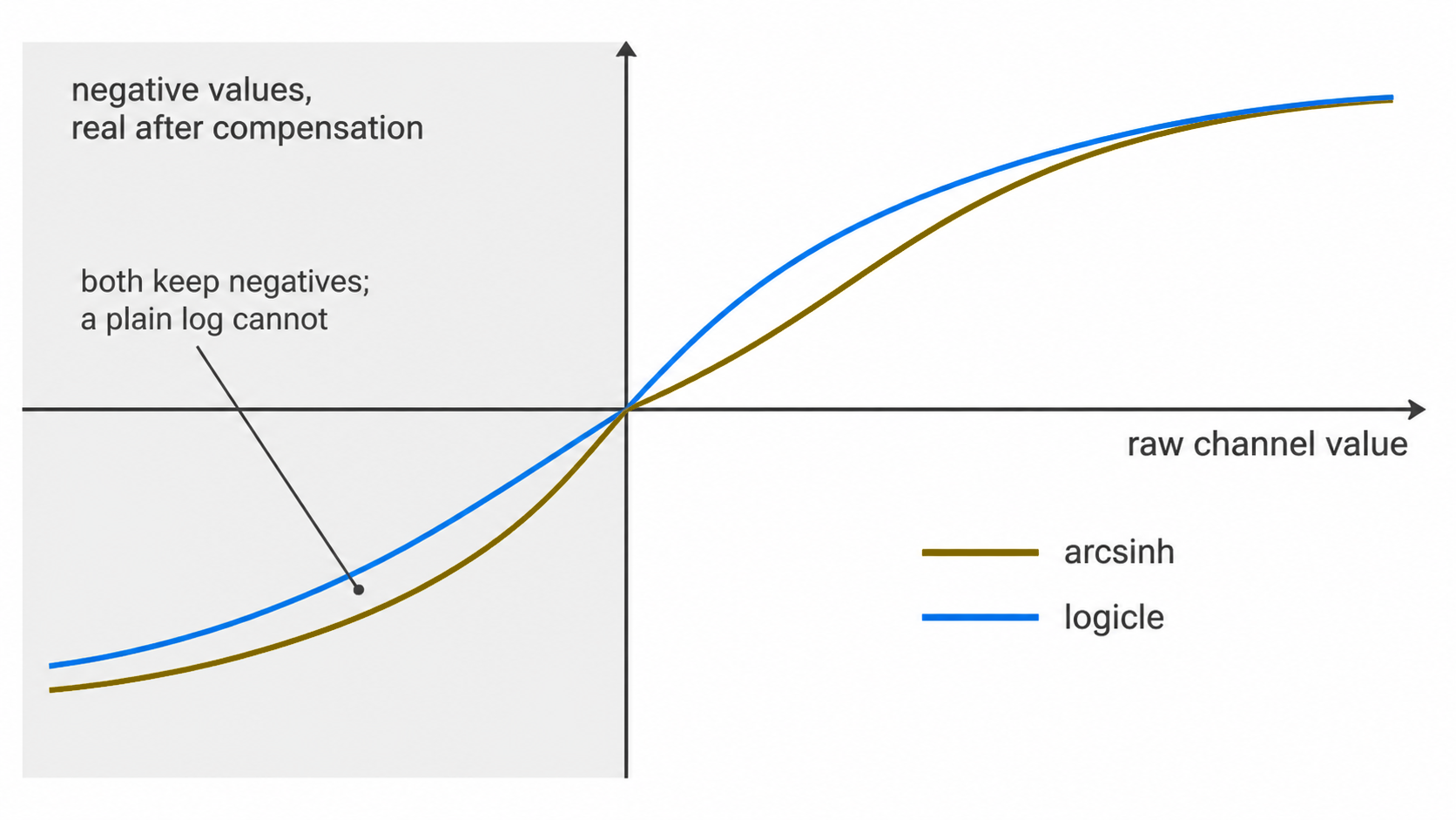
Fluorescence intensities span four to five decades. Untransformed, the negative population compresses against the axis and mode separation is not resolvable. Every threshold in section 2 is therefore placed on a transformed scale, and the choice of transform determines where it lands.
4.2 Arcsinh
The default. The cofactor governs the width of the quasi-linear
region near zero and is estimated per panel by bisection until the
interquartile range of the background distribution reaches a target,
which puts it near 1.6 standard deviations of a negative population:
just wider than the negatives, the condition under which a symmetric
negative population stays one mode. This is a heuristic rather than a
published criterion. The conventional value of 5 derives from mass
cytometry and over-expands the background band on spectrally unmixed
fluorescence data, so it is estimated rather than assumed.
derive_cofactor_pooled() estimates across samples so that a
single weakly stained file does not set the scale for the batch, and on
the scatter-gated single cells rather than every event, so debris does
not set the background (--cofactor-from-all-events restores
the older estimate).
One cofactor serves every marker by default. Detectors differ
many-fold in how wide their negatives are, and a cofactor per channel is
the published recommendation for flow data (den Braanker et al. 2021;
Azad et al. 2016). --per-marker-cofactor gives each marker
its own, estimated by the same criterion on that marker’s negative
population, reconstructed from its values below zero. It is not the
default. On a whole-blood cohort scored against manual gating it ranked
samples no better (mean Spearman rho 0.64 for both), its worst-sample
errors were larger and one more file failed staining QC, and on a PBMC
cohort it emptied CD4 T cells in 3 of 30 samples and regulatory T cells
and NKT cells in 6 each. Logicle, which fits its width per channel,
scored the same as the shared cofactor on the whole-blood cohort and
emptied regulatory T cells in 4 of the PBMC samples against 1. A small
per-channel cofactor stretches the background differences between cell
types, which leaves more markers without a density minimum.
4.3 Logicle
--transform logicle implements the automatic logicle
rule with linearisation width w = (m -
log10(t/|r|))/2, where r is the
fifth percentile of the negative values and t the top of the
channel’s declared range. Both transforms are linear near zero and both
represent compensated negative values; arcsinh is defined for every real
number and is a Gating-ML scale like logicle (Spidlen et al. 2015). What
logicle adds is that the width of its linear region is fitted per
channel to that channel’s negatives (Parks et al. 2006), which arcsinh
does only under --per-marker-cofactor.
Parameters are pooled across the panel. Per-file fitting, implemented by some tools, assigns each sample an independent scale and invalidates cross-sample comparison of medians.
4.4 Consequence
The transform is not a display parameter. On a seven-colour T cell panel, lineage-level populations agreed within 0.1% between transforms while CCR7 and CD45RA memory subsets differed by tens of percent.
The mechanism is recorded in thresholds_used.csv. Under
arcsinh the CCR7 threshold resolved to a density minimum in some samples
and to a quantile fallback in others, a difference of approximately 2.5
units on that scale. Under logicle a minimum was resolved in every
sample. For dim markers without clear bimodality the transform
determines whether a stable threshold exists at all, which makes the
source column a prerequisite for interpreting any memory
subset frequency.
--transform none bypasses transformation for
pre-transformed input.
5. Compensation
Fluorochrome emission spectra overlap, so signal from one dye is registered in detectors assigned to others. Uncorrected, this produces apparent positivity in channels the cell does not express.
The spillover matrix is determined at acquisition from single-stain
controls and stored in the FCS keyword block. cyRAVEN applies it where
present and reports its absence. Spectral instruments write unmixed data
with no matrix, so maybe_compensate() detects rather than
assumes, since applying compensation twice is as damaging as omitting
it.
Matrix construction is out of scope. It belongs in acquisition software, where the single-stain controls can be inspected.
5.1 What compensation cannot undo
Subtracting a fluorochrome’s expected contribution to another
detector is correct on average. What the subtraction cannot remove is
the photon-counting variance that came with the contribution, so a
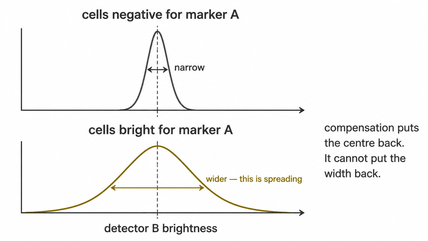
channel receiving spillover from a bright neighbour has a negative
population that is correctly centred and abnormally wide. Two modes that
were separable merge, the valley fills in, and section 2.3 reports a
tail gate (tailgate) with no indication of why.
spreading_receivers.csv supplies the cause. For each
ordered channel pair, the spread of the receiver’s negative population
is compared between cells negative and positive for the source;
restricting to the receiver’s own negatives is what makes this spreading
rather than biology, since co-expression moves the positive cells and
not the width of the negatives. spreading_pairs.csv holds
the full pairwise ranking.
The finding to act on is the join between the two: a marker that both shows no density minimum in most samples and receives substantial spreading is reported as a panel design problem. No gating strategy recovers a cut that spreading has erased.
This is a ranking computed from the samples in hand, not a spillover
spreading matrix. The published SSM is derived from single-stain
controls, and the values here are not comparable with it; given those
controls with --single-stains, the package computes it
(spillover_spreading_matrix.csv).
spreading_pairs.csv also screens for compensation
errors. Correct compensation leaves the receiver’s median where it is as
the source brightens, so trend_rho, the rank correlation
between the two among source-positive cells negative for the receiver,
is flagged possible_compensation_error at 0.3 or more in
size, a conventional cut rather than a validated one. A negative trend
on a pair whose receiver is also wider at a given source level is
reported as trend_unresolved instead: the screen reads only
cells below the receiver’s cut, and brighter source cells, with the
wider receiver distribution, lose more of it to that cut, which pulls
the trend negative with compensation correct. Single-stain controls
decide such a pair.
Commands and every option
One page for every way to run the pipeline: the commands for each task, in Docker and in R, and every option with the situation it is for.
Part 1 is the commands. Part 2 is how to choose between the options that matter. Part 3 is the exhaustive reference.
Part 1. Commands
1.1 Docker or R
Both call the same run_cyraven(). The command-line front
end is
system.file("scripts", "cyraven.R", package = "cyRAVEN"),
which is what the container entrypoint executes.
| Docker | R | |
|---|---|---|
| Use it when | Results will be published, shared or compared against another machine | Developing, exploring, or Docker is unavailable |
| Reproducible | Yes: R 4.4.3, a dated CRAN snapshot and Bioconductor 3.20 are pinned | Only against your own library |
| Option syntax | --group-column cohort |
group_column = "cohort" |
| Paths | Inside the container | On the host |
Every option name is the same in both. Replace hyphens with
underscores: --group-column becomes
group_column =. Flags that take no value become
TRUE: --cluster becomes
unsupervised = TRUE.
docker run --rm cyraven:1.0.0 --help prints the list at the
version installed.
1.2 Get the image, once
See Setup. Pull for a released run, build for a modified source tree, and pin the version for anything you intend to publish.
1.3 A first run on a new cohort
Each step is cheap and catches what the next would otherwise waste time on. Every block below is one command, meant to be copied on its own and run before the next is copied. Steps 2 and 4 are edits you make in a text editor, not commands, which is the other reason these are not one block: copying a numbered list of commands and comments into a terminal in one go runs them all before you have looked at anything.
1. Make the folders and put the FCS files in
data/fcs/.
2. Write a sheet with a row for every file.
docker run --rm \
  -v "$PWD/data:/data" \
  cyraven:1.0.0 \
  --dir /data/fcs \
  --recursive \
  --write-samples /data/samples.csv
3. Edit data/samples.csv and fill in
patient_id, cohort and any study variable. No
command; open it in a spreadsheet or a text editor.
4. Start the config from the shipped template.
5. Edit populations: in
data/analysis.yaml to match your panel. Again an
edit, not a command.
6. Validate, in seconds, analysing nothing.
docker run --rm \
  -v "$PWD/data:/data:ro" \
  -v "$PWD/results:/results" \
  cyraven:1.0.0 \
  --dir /data/fcs \
  --recursive \
  --samples /data/samples.csv \
  --config /data/analysis.yaml \
  --outdir /results \
  --check
7. Repeat steps 5 and 6 until --check
reports no problems. Then run it.
docker run --rm \
  -v "$PWD/data:/data:ro" \
  -v "$PWD/results:/results" \
  cyraven:1.0.0 \
  --dir /data/fcs \
  --recursive \
  --samples /data/samples.csv \
  --config /data/analysis.yaml \
  --group-column cohort \
  --reference-group "Healthy controls" \
  --outdir /results
8. Open results/report.html.
The two input files are described in the Inputs.
In R:
library(cyRAVEN)

opt <- list(
  dir = "data/fcs", recursive = TRUE,
  outdir = "results/",
  samples = "data/samples.csv",
  config = "data/analysis.yaml",
  group_column = "cohort",
  reference_group = "Healthy controls",
  seed = 42)

# validate
run_cyraven(c(opt, list(check_only = TRUE)))
# run
run_cyraven(opt)
1.4 The full analysis
Batch diagnostics and the unsupervised check are opt-in because each adds outputs and runtime.
docker run --rm \
  -v "$PWD/data:/data:ro" \
  -v "$PWD/results:/results" \
  cyraven:1.0.0 \
  --dir /data/fcs \
  --recursive \
  --samples /data/samples.csv \
  --config /data/analysis.yaml \
  --group-column cohort \
  --reference-group "Healthy controls" \
  --batch-column acquisition_date \
  --cluster \
  --covariates age,sex \
  --reference-date 2025-01-01 \
  --no-session \
  --outdir /results
1.5 A cohort that must fit in memory
Peak memory is set by the events held at once, not by the number of files.
docker run --rm \
  -v "$PWD/data:/data:ro" \
  -v "$PWD/results:/results" \
  cyraven:1.0.0 \
  --dir /data \
  --recursive \
  --samples /data/samples.csv \
  --config /data/analysis.yaml \
  --max-events-per-file 300000 \
  --cells-per-sample 6000 \
  --max-cells 150000 \
  --no-session \
  --outdir /results
Run one analysis at a time. The stages are already multi-threaded, so nothing is gained by running containers in parallel, and two concurrent runs at these settings will exhaust a workstation. A run killed by the out-of-memory killer exits 137 and writes no report, because SIGKILL runs no handler.
Subsampling raises every detection limit in proportion, because it lowers the parent-gate count each frequency is a fraction of.
1.6 Comparing runs over time
Once, on the run being adopted as the reference.
docker run --rm \
  -v "$PWD/data:/data:ro" \
  -v "$PWD/results:/results" \
  cyraven:1.0.0 \
  --dir /data/fcs \
  --samples /data/samples.csv \
  --config /data/analysis.yaml \
  --outdir /results \
  --write-baseline /results/baseline.rds
On every later run.
docker run --rm \
  -v "$PWD/data:/data:ro" \
  -v "$PWD/results2:/results" \
  -v "$PWD/results:/prev:ro" \
  cyraven:1.0.0 \
  --dir /data/fcs \
  --samples /data/samples.csv \
  --config /data/analysis.yaml \
  --outdir /results \
  --baseline /prev/baseline.rds \
  --fail-on-drift
--fail-on-drift exits non-zero after every output has
been written, so it can gate a pipeline without costing the diagnostics
that explain the failure.
1.7 The demonstration cohort
See Quick start. Nothing is downloaded: the data ship inside a package cyRAVEN already depends on, so the example is reproducible offline.
1.8 Iterating on the code
Mount a checkout and set CYRAVEN_SOURCE; the entrypoint
loads that tree through pkgload::load_all() instead of the
installed copy, so edits take effect without a rebuild.
1.9 Paths, mounts and platforms
Every path inside a flag is a path inside the container.
--outdir must fall within a mounted volume or the output is
discarded when the container exits.
| Platform | Substitution |
|---|---|
| Linux, macOS | as written |
| Windows PowerShell |
${PWD} for $PWD
|
| Git Bash on Windows | prefix MSYS_NO_PATHCONV=1, or the shell rewrites
/data into a Windows path |
Mount the data read-only (:ro) so a bug cannot alter raw
acquisition files.
Part 2. Which option to use when
2.1 The rule behind the defaults
Options fall into three classes, and the class fixes the default.
Additive. Produces a new output and alters nothing
existing. The diagnostics are on by default, because an analysis that
has to be requested is one that does not get run, and the
--no-* flags switch them off. Secondary or exploratory
analyses (--cluster, --explore,
--edger, --rank-ancova) and the exports are
asked for.
Parametric. Changes how an existing quantity is computed. Defaults are the values the pipeline was validated with; changing one changes results and is a decision to record.
Consequential. Changes numbers a previous run
reported, by design. Off by default without exception, and recorded in
run_manifest.txt when used. They are
--transform, --per-marker-cofactor,
--adaptive-gates, --peer-cuts (and
--auto-fix-gates, which implies it),
--drop-unstable-events, --peacoqc,
--subsample rare, --correct-batch and
--calibration-beads.
2.2 Choosing by situation
Each of the following is a complete command. $D is the
mount pair every run needs, written once here so the recipes stay
readable:
or write the two -v flags out in full, as in Part 1.
Most thresholds found no density minimum
thresholds_used.csv shows source = tailgate
(or quantile_fallback) on most rows. The marker did not
separate positive from negative, so the cut carries no evidence of
separation. Try the transform first, because for dim markers it decides
whether a stable threshold exists at all.
docker run --rm $D \
  cyraven:1.0.0 \
  --dir /data/fcs \
  --samples /data/samples.csv \
  --config /data/analysis.yaml \
  --transform logicle \
  --group-column cohort \
  --reference-group "Healthy controls" \
  --outdir /results
If it persists, declare an unstained or fluorescence-minus-one
control in the sheet (is_control, fmo_for) so
the cut has a reference rather than a guess. If it still persists, the
marker is not resolving in this panel and no gating strategy recovers
it; spreading_receivers.csv says whether the optics explain
it. --transform is consequential: it moves every threshold,
so say so when reporting.
A population may exist that the specification does not describe
The declared populations are only ever what was declared. Clustering is the one output that can contradict them.
docker run --rm $D \
  cyraven:1.0.0 \
  --dir /data/fcs \
  --samples /data/samples.csv \
  --config /data/analysis.yaml \
  --cluster \
  --explain-clusters \
  --group-column cohort \
  --reference-group "Healthy controls" \
  --outdir /results
--cluster writes
cluster_gate_agreement_*.csv: a cluster dominated by no
declared label is a population the specification misses, and a label
spread across many clusters covers several phenotypes.
--explain-clusters then learns a two-marker gating strategy
for each undescribed cluster and writes
cluster_gate_proposals.csv. It is descriptive: it proposes
gates and never changes a scored one. Promoting a proposal to a named
population is a manual edit to the config, and the next run reads
it.
Samples were acquired on several days or instruments
docker run --rm $D \
  cyraven:1.0.0 \
  --dir /data/fcs \
  --samples /data/samples.csv \
  --config /data/analysis.yaml \
  --batch-column acquisition_date \
  --group-column cohort \
  --reference-group "Healthy controls" \
  --outdir /results
This quantifies the batch structure without altering anything: iLISI against a permutation null, per-marker distributional drift, and Cramér’s V between batch and group.
Read batch_group_confounding.csv before going
further. If V is high, the batches and the groups are
the same partition, and correcting the batch removes the finding.
cyRAVEN refuses correction above Cohen’s large association for the
table’s size, 0.5/√(k − 1) with k the smaller of the batch and group
counts (0.5 for two groups), for that reason. Where V is low
and the drift is real, add correction:
docker run --rm $D \
  cyraven:1.0.0 \
  --dir /data/fcs \
  --samples /data/samples.csv \
  --config /data/analysis.yaml \
  --batch-column acquisition_date \
  --correct-batch \
  --group-column cohort \
  --reference-group "Healthy controls" \
  --outdir /results
--correct-batch is consequential. It applies to the
embedding and clustering, not to per-sample thresholds, which are
batch-local by construction.
Absolute cell numbers rather than percentages
A frequency is a proportion of a parent gate, so it moves whenever
any other population moves. Add count.<Population>
columns to the sheet, in cells per microlitre, and the run tests them
alongside the frequencies:
file,sample_id,cohort,count.Monocytes
HC-01.fcs,HC-01,Healthy controls,420
docker run --rm $D \
cyraven:1.0.0 \
--dir /data/fcs \
--samples /data/samples.csv \
--config /data/analysis.yaml \
--group-column cohort \
--reference-group "Healthy controls" \
--outdir /resultsNo extra flag: the columns are recognised by their prefix.
absolute_counts_qc.png draws every supplied count as one
tile per sample and population on a log scale, which is how a
transcription error (a tile decades off its column) or a name mismatch
(a missing row) is caught. Where the counting instrument exports its own
sheet and transcription is not worth it, use
--absolute-counts <file> instead.
The same assay runs repeatedly and must not drift
Record where the accepted run placed its thresholds:
docker run --rm $D \
  cyraven:1.0.0 \
  --dir /data/fcs \
  --samples /data/samples.csv \
  --config /data/analysis.yaml \
  --outdir /results \
  --write-baseline /results/baseline.rds
Then test every later run against it:
docker run --rm $D \
  cyraven:1.0.0 \
  --dir /data/fcs \
  --samples /data/samples.csv \
  --config /data/analysis.yaml \
  --outdir /results \
  --baseline /results/baseline.rds \
  --fail-on-drift
The within-run peer check already finds one deviant tube among its
peers. It cannot find a cohort that moved as a whole, because the peer
median moves with it; only a baseline from an earlier run can.
--fail-on-drift exits non-zero after every output has been
written, so it can gate a pipeline without costing the diagnostics that
explain the failure. Omit it while investigating.
A longitudinal or paired design
docker run --rm $D \
  cyraven:1.0.0 \
  --dir /data/fcs \
  --samples /data/samples.csv \
  --config /data/analysis.yaml \
  --paired-column patient_id \
  --condition-column timepoint \
  --group-column cohort \
  --reference-group "Healthy controls" \
  --outdir /results
Both flags are required together. Pairing is never inferred: a design where each donor appears twice is indistinguishable, from the data alone, from one where two donors happen to share a label, and guessing wrong changes every p-value.
The same two flags also produce
population_trajectories.png: one line per patient across
the conditions, with the cohort median drawn over them. Add
--clinical-columns survival_28d and the lines are coloured
by outcome, which is the comparison a longitudinal design is usually
about. Survivors and non-survivors often differ in the direction each
patient moves rather than at any single timepoint, and a box per
timepoint averages exactly that away.
A cohort with clinical scores and outcomes
C=sofa,survival_28d,crp_mg_l,age_years
docker run --rm $D \
  cyraven:1.0.0 \
  --dir /data/fcs \
  --samples /data/samples.csv \
  --config /data/analysis.yaml \
  --group-column infection_focus \
  --reference-group Pulmonary \
  --clinical-columns "$C" \
  --outdir /results
Any sheet column can be named. sofa and
crp_mg_l are numeric and get Spearman’s rho,
survival_28d has two levels and gets Wilcoxon with Cliff’s
delta, and each effect is written with a percentile bootstrap interval.
On a cohort of ten that interval usually spans zero, meaning the effect
is not resolved. Read clinical_variables_correlation.png
first: p-values are adjusted within each variable on the assumption that
the variables are separate questions, and two variables correlated with
each other are one question asked twice.
One sample’s threshold is visibly wrong
Where gating_qc.png shows the derived cut sitting in a
shoulder for one sample only, correct that sample rather than pinning
the marker for all of them. In the config:
sample_overrides:
  PT-01_v1:
    CD14:
      threshold: 2.4
      set_by: "your initials"
      reason: >-
        bimodal but the minimum fell in
        the shoulder, see gating_qc.png
Then run normally. set_by and reason are
recorded in run_manifest.txt, so a run touched by hand says
so in its provenance rather than only in the table it altered. Setting a
fixed threshold for every sample instead would reintroduce the
fixed-coordinate bias the pipeline exists to remove.
A rare population is invisible in the embedding
Uniform sampling reproduces each sample’s composition, so a population at 0.1% contributes 0.1% of the drawn cells and forms no cluster.
docker run --rm $D \
  cyraven:1.0.0 \
  --dir /data/fcs \
  --samples /data/samples.csv \
  --config /data/analysis.yaml \
  --subsample rare \
  --cluster \
  --group-column cohort \
  --reference-group "Healthy controls" \
  --outdir /results
Consequential: it changes which cells are embedded, so the UMAP is
not comparable with a uniform run, and cells_umap.csv gains
a sampling_weight column. Frequencies are unaffected,
because they are computed on all events rather than on the drawn
subset.
Gates are needed on the instrument or in FlowJo
docker run --rm $D \
  cyraven:1.0.0 \
  --dir /data/fcs \
  --samples /data/samples.csv \
  --config /data/analysis.yaml \
  --cluster \
  --explain-clusters \
  --export-gates \
  --flowjo-export \
  --outdir /results
--export-gates writes ISAC Gating-ML 2.0 on the scale
the gates were fitted on, through its fasinh or
logicle transformation, with each dimension named by the
files’ $PnN; and a vertex table in the linear units the FCS
file stores, edges subdivided so the polygon describes the same region
the fit did. To apply a file whose gates reference the files’ own
compensation (compensation-ref="FCS") with flowCore and
flowUtils, use flowCore 2.25 or later, or the cyRAVEN image, whose
flowCore 2.18.0 carries the one-line fix: releases 2.18 to 2.22 stop on
R 4.2 or later when they read a $SPILLOVER keyword (“the
condition has length > 1”). --flowjo-export writes
UMAP-annotated FCS: open _ALL_SAMPLES.fcs, plot UMAP-1
against UMAP-2, and the populations are there as channels.
Intensities must be comparable across instruments or over months
docker run --rm $D \
  -v "$PWD/beads:/beads:ro" \
  cyraven:1.0.0 \
  --dir /data/fcs \
  --samples /data/samples.csv \
  --config /data/analysis.yaml \
  --calibration-beads /beads/rainbow.fcs \
  --calibration-values /beads/lot.csv \
  --outdir /results
Consequential, and the most far-reaching of them: conversion happens
before any threshold is derived, so every intensity in the run changes
units. A channel whose fit falls below --calibration-min-r2
is left in instrument units rather than converted on a fit that does not
hold, and the log says which.
Labels from another tool
docker run --rm $D \
  cyraven:1.0.0 \
  --dir /data/fcs \
  --samples /data/samples.csv \
  --config /data/analysis.yaml \
  --external-labels /data/labels.csv \
  --export-gates \
  --outdir /results
Learns a gating strategy per supplied label and measures whether it
holds on donors it was not fitted to. Held-out events from the same
donors overstate how well a gate travels; the per-donor minimum in
gate_transferability.csv does not. See Interoperability.
The run is slow, or the machine runs out of memory
In this order, because the first costs nothing analytically:
Skip the session file: often most of the wall-clock, none of the results.
docker run --rm $D \
  cyraven:1.0.0 \
  --dir /data/fcs \
  --samples /data/samples.csv \
  --config /data/analysis.yaml \
  --no-session \
  --outdir /results
Bound the events read per file, then the cells embedded.
docker run --rm $D \
  cyraven:1.0.0 \
  --dir /data/fcs \
  --samples /data/samples.csv \
  --config /data/analysis.yaml \
  --no-session \
  --max-events-per-file 300000 \
  --cells-per-sample 6000 \
  --max-cells 150000 \
  --outdir /results
--no-session changes no number.
--max-events-per-file does: it raises every detection limit
in proportion, because it lowers the parent-gate count each frequency is
a fraction of. Run one analysis at a time; the stages are already
multi-threaded.
You suspect the specification is missing something
The declared path scores what you declared. It cannot find a population nobody wrote down, and it cannot see outside the parent gate. Explore mode is the complement: every event, every eligible channel, no specification.
Alongside the declared analysis. Writes to results/explore/ and changes NOTHING in the existing output.
docker run --rm $D \
  cyraven:1.0.0 \
  --dir /data/fcs \
  --samples /data/samples.csv \
  --config /data/analysis.yaml \
  --group-column cohort \
  --reference-group "Healthy controls" \
  --cluster \
  --explore \
  --outdir /results
…and let the two sides inform each other. The declared run lends explore its per-sample thresholds, so clusters are NAMED rather than guessed at; explore lends the declared run spec_gaps.csv, naming populations that span several clusters and clusters nothing covers.
docker run --rm $D \
  cyraven:1.0.0 \
  --dir /data/fcs \
  --samples /data/samples.csv \
  --config /data/analysis.yaml \
  --group-column cohort \
  --reference-group "Healthy controls" \
  --cluster \
  --explore \
  --maybe-learn \
  --outdir /results
Without --maybe-learn the two are computed in complete
isolation, which is the right default: a check on the specification has
to be independent of the specification to be worth anything.
A new panel, and no specification written yet
# No --config and no --samples:
# a folder of FCS files is the whole input.
docker run --rm $D \
  cyraven:1.0.0 \
  --dir /data/fcs \
  --explore-only \
  --outdir /results
Read results/explore/explore_report.html, then curate
results/explore/explore_suggested_spec.yaml into a real
specification and run the supervised path with it. Full detail in Explore
mode.
2.3 The options that change reported numbers
Turn these on only when you mean to, and say so when you report a result.
| Option | What it changes | Read first |
|---|---|---|
--transform logicle |
Every threshold, and therefore every frequency | gating_qc.png |
--per-marker-cofactor |
Every threshold on an arcsinh scale | gating_qc.png |
--adaptive-gates |
Thresholds, wherever another rule scores a better gap |
thresholds_used.csv (source),
gating_qc.png
|
--peer-cuts, --auto-fix-gates
|
The cuts and hierarchy gates they replace or skip | gate_adjustments.csv |
--drop-unstable-events |
Every count in an affected file | acquisition_qc_impact.csv |
--peacoqc |
Every count in a file PeacoQC flags | peacoqc_summary.csv |
--subsample rare |
Which cells are embedded |
cells_umap.csv gains sampling_weight
|
--correct-batch |
Marker values in the embedding and clustering | batch_group_confounding.csv |
--calibration-beads |
The units every intensity is expressed in | calibration.csv |
2.4 What not to change without cause
--cofactor is estimated per panel for a reason: the
conventional value of 5 comes from mass cytometry and over-expands the
background band on unmixed fluorescence.
--batch-max-cramers-v exists to refuse correction where
batch and group are inseparable. Raising it, or passing
--force-batch-correction, means the resulting difference
cannot be attributed to biology.
Pinning a threshold in the config applies it to every sample and
reintroduces the fixed-coordinate bias the pipeline exists to remove.
Use sample_overrides: for one sample instead.
Part 3. Every option
The same names are the element names of the list passed to
run_cyraven(), with hyphens replaced by underscores.
3.1 Input
| Option | Default | Effect |
|---|---|---|
--files |
none | Comma-separated paths, or a glob in quotes |
--dir |
none | Directory to search for .fcs. Alternative to
--files
|
--recursive |
off | Search --dir recursively, for cohorts in
subdirectories |
--pattern |
[.]fcs$ |
Regex for filenames under --dir. Any file containing
.fcs that fails the pattern is listed as a warning rather
than silently skipped |
--exclude |
compensation controls | Regex; matching paths are dropped after discovery. The default
removes single-stain setup files, which carry no CD45 population and
form a spurious panel group. --exclude '' keeps
everything |
--max-events-per-file |
0, meaning all | Read at most N events per file, sampled evenly through the acquisition rather than taken from the start. Bounds peak memory, and raises every detection limit in proportion because it lowers the parent-gate count |
--outdir |
results |
Output directory |
3.2 Inputs and metadata
The standard input is one CSV and one YAML. The three separate tables
below them still work unchanged and are not deprecated, but cannot be
combined with --samples. See the Inputs.
| Option | Default | Effect |
|---|---|---|
--samples |
none | The sample sheet: one row per FCS file carrying its identity, its
subject’s attributes, its study variables and any
count.<Population> columns. Replaces the three
options below |
--config |
built-in spec | The analysis: population specification,
functional_blocks, ratios, threshold and
sample_overrides, colours, metadata dictionaries, and the
samples: section naming which sheet column plays which
role |
--write-samples |
none | Write a sheet template covering every input file, and exit |
--check |
off | Validate the inputs from FCS headers alone and exit. Reports resolved markers, specification entries matching none of them, sheet coverage, group levels and sizes, batches and study variables. Seconds rather than the full run |
--list-channels |
off | List every acquisition parameter and exit: index, $PnN,
$PnS, and the symbol the run resolves it to, which is the
name the specification must use. Also reports whether every file carries
the same panel. Needs no sheet and no config, because it answers what to
put in one |
--ignore-channels |
none | Comma-separated marker names dropped before anything else, including
before the panel fingerprint. Names match whole and case-insensitively;
a name containing * is a glob. See A channel that splits the
cohort
|
--reference-date |
today |
YYYY-MM-DD used to derive age from date of birth and to
place two-digit years. Set it to a fixed study date so ages do not
change between runs |
--group-column |
resolved cohort
|
Column defining the comparison groups. Enables the between-group
figure and tests. Also settable as samples: group_column:
in the config, which the flag overrides |
--reference-group |
first alphabetically | The group every other is tested against. Drawn unfilled and leftmost |
--write-config |
none | Derive everything, write the resulting YAML, and exit. Shows what
the pipeline detected before time is spent. The per-sample cuts are
summarised under thresholds_derived, which no run reads; a
value copied into thresholds: is applied to every sample.
Needs --outdir as well: deriving the
parameters means reading the files, so the early stages run and write
their QC output alongside |
The earlier three-file form:
| Option | Default | Effect |
|---|---|---|
--sample-map |
none | CSV linking each filename to a sample, patient, group and control
status. Only file is required. Also carries
fmo_for and control_group
|
--patient-table |
none | Clinical covariates keyed on patient identifier. Supplies
wbc_per_ul for absolute concentrations |
--absolute-counts |
none | Externally measured absolute counts, wide format. Requires
--sample-map
|
--write-sample-map |
none | Write a sample-map template and exit |
A channel that splits the cohort
The panel fingerprint is the set of marker names a file resolves. Files sharing a set form one panel, and each panel gets its own cofactor, its own embedding and its own thresholds. That is correct when panels differ, and destructive when they do not.
Spectral unmixing is where it usually goes wrong. Unmixing writes the
extracted autofluorescence back as channels, often named
[AF color 1] and upward, and how many it writes depends on
the sample rather than on the panel. They are not stains and nothing is
measured with them, but they enter the fingerprint like any other
channel, so twelve comparable files can resolve into seven panels of one
or two files each. Every downstream quantity is then derived within a
panel of one, and nothing is comparable to anything.
--list-channels shows the resolved names, and
--check reports markers that are not present in every file.
When the culprit is a nuisance channel, drop it:
The channel is removed before the fingerprint is taken, so the files
collapse back into one panel. Names match whole and case-insensitively,
and * makes an entry a glob, so CD16 matches
CD16 and not CD161. Separate several with
commas.
Only drop a channel that carries no signal you intend to use. A real marker missing from some files is a different problem, and the honest handling of it is the panel split.
3.3 Transformation and gating
| Option | Default | Effect |
|---|---|---|
--transform |
arcsinh |
arcsinh, logicle or none.
Consequential: it moves every threshold. For dim
markers it decides whether a stable threshold exists at all |
--cofactor |
derived per panel | Fixed arcsinh cofactor. The conventional value of 5 comes from mass cytometry and over-expands the background band on unmixed fluorescence, which is why it is estimated rather than assumed |
--cofactor-from-first-sample |
off | Derive the cofactor from the first file only, as before pooling was introduced |
--per-marker-cofactor |
off | One arcsinh cofactor per marker, from the spread of that marker’s negative population, instead of one for the panel. Consequential: it moves every cut. See section 4.2 |
--cofactor-from-all-events |
off | Estimate the cofactor over every event, debris included, instead of the scatter-gated single cells |
--keep-margin-events |
off | Keep events at the top of a marker or scatter channel’s range,
capping their values, instead of removing them. Counts are in
margin_events.csv either way |
--spillover |
none | CSV spillover matrix applied to every file in place of its own
$SPILLOVER
|
--fmo-sets-cut |
off | Let a true FMO set the cut even where the sample’s valley is higher,
so dim positives between them count as positive
(fmo_q995_valley_lowered). Off by default because an FMO
argues a cut down validly only where its negative is the sample’s own,
and one tube serves every sample of its panel or
control_group; a valley below the FMO’s edge is raised to
it either way. Never applied to unstained or minus-multiple tubes |
--logicle-m |
4.5 | Decades on the logicle display scale |
--singlet-mad-k |
3 | How far below the FSC-H:FSC-A ridge, in MADs, the singlet gate cuts. One-sided, because doublets have a low ratio. The gate is skipped, with a log line, when the two are not distinct channels |
--viability-marker |
auto-detect | Name the dye where the pattern is ambiguous |
--min-cd45-pct |
5 | Staining QC floor, percent CD45+ of live |
--min-live-pct |
unset | The assay’s minimum live share of single cells, in percent; a sample
below it fails staining QC. Unset, the share is reported in
staining_qc.csv and not judged, because no published
minimum exists. A sample whose dead cells outnumber its live ones reads
as mostly live: the viability cut is placed above the dye’s tallest
mode, which is then the dead cells.
pct_live_if_dominant_dead beside it gives the live share
for that case, from a dye minimum below the dominant mode |
--include-qc-failed |
off | Keep declared samples that failed staining QC. Admits them to every
stage, not only the embedding. Their percentages carry no evidence;
under this flag qc_status reads pass and only
the verdict column in staining_qc.csv records
which were forced in |
--discover-controls |
off | Let a sample that fails staining QC become the unstained reference for its panel even though the sheet declares no control. See below for why this is off |
--adaptive-gates |
off | Choose each threshold by sweeping the kernel bandwidth and trying the tail and Otsu rules, instead of one fixed smoothing with a tail-gate fallback. Consequential: it moves thresholds. See Placing a threshold when no valley exists |
--peer-cuts |
off | Where a population marker shows a density minimum in most samples of
a panel but not in this one, take this sample’s cut from the median of
those minima; where most samples show none, replace only a quantile
fallback or a tail cut far from the others. Each change is a row of
gate_adjustments.csv, and the original cut stays in
derived_threshold. Consequential: it moves
thresholds. Implied by --auto-fix-gates
|
--panel-optional-markers |
none | Comma-separated markers that do not define the panel. A reagent stained in only some files otherwise splits the cohort into separate panels with separate embeddings. Named here, the files stay one panel; a population needing the marker scores where it exists and is UNAVAILABLE where it does not |
Placing a threshold when no valley exists
density_valley() answers one question: where is the
deepest separation between two modes that counting noise cannot explain.
Where a marker shows none it answers NA, and the threshold
then comes from the tail gate, 3.5 robust standard deviations above the
dominant mode and flagged for review; a fixed quantile of the parent
remains only where no tail gate can be placed.
Before the tail gate that quantile was the default, and on a spectral
panel it was not a rare outcome. On the sepsis cohort this was written
against, 65% of every sample-by-marker cut came back
quantile_fallback, which means two thirds of the gates were
placed by the constant rather than by the data, and the viability gate
was skipped in all 20 samples because L/D never resolved.
The markers were not unimodal. The histogram being smoothed (220 bins, a 9-bin moving average) is under-smoothed for these data: L/D showed 32 peaks in one sample and CD45 showed 10, nearly all of them noise. Widen the kernel and CD45 resolves to exactly two modes.
--adaptive-gates keeps the same vocabulary as openCyto
(Finak and
others, 2014) rather than inventing one:
| Method | For |
|---|---|
| mindensity over a bandwidth ladder | a bimodal marker, at whatever smoothing resolves it |
| tailgate | one real mode with a positive tail. The cut sits a robust spread above the mode, estimated by mirroring the half the tail cannot reach |
| Otsu | two classes of comparable size |
Every candidate is then scored the same way: how deep a density gap the cut sits in. That is method-agnostic, needs no per-marker configuration, and measures the property a gate is supposed to have. Where nothing sits in a gap the tail rule is preferred over the quantile, because it is anchored to the sample’s own mode and spread rather than declaring a fixed share positive.
Measured on that cohort: quantile fallbacks fell from 65% to under 1% on properly gated data, and the viability gate placed at 0.1 to 2.4% dead.
It cannot find a population that was not stained. One sample there carries CD3 at 0.3% positive while its CD45 stains normally. No threshold rule recovers T cells from a channel holding none, and the selector reports what is there.
Do not require the parent marker twice
A specification that opens every population with
CD45: above looks like the textbook leukocyte gate and is a
trap.
The hierarchy has already applied CD45: the parent every population
is scored inside is cd45_pos. Repeating the requirement
asks for a second CD45 threshold derived from the cells that passed the
first. In PBMC that distribution is all positive and unimodal; in whole
blood its one minimum separates the CD45-dim granulocytes from the
CD45-bright lymphocytes, and above then removes the
granulocytes from every population that names it. Either way the second
cut describes nothing the specification meant.
When single-mode cuts fell back to the 90th percentile, an
above comparison kept exactly 10%. On the cohort above,
CD45 fell back to the quantile in 17 of 20 samples and the share of
parent cells carrying any label came out at 10.0, 9.4, 9.3, 9.8 and 9.5%
for the first five. Removing the redundant requirement took classified
cells from 21% to 88%. Nothing else about the
specification changed. The tail gate that now replaces the quantile goes
above the dominant mode unless the marker is declared
tail: lower, so on PBMC, where every parent cell is
CD45-positive, the repeated requirement now keeps almost nothing.
The rule generalises: do not name a marker in a population if a gate above it has already applied that marker.
3.4 Uncertainty and detection limits
| Option | Default | Effect |
|---|---|---|
--no-uncertainty |
on | Skip the gate placement uncertainty analysis, and with it the
detection limits (lod_pct, loq_pct,
detection), which are computed in the same pass |
--uncertainty-boot |
100 | Bootstrap replicates per threshold. Below about 50 the standard uncertainty is itself noisy |
--uncertainty-max-events |
20000 | Events per replicate. The cut is a histogram feature and stops moving well before the whole parent gate is used |
--lod-events |
20 | Events below which a population is reported below the limit of detection |
--loq-events |
50 | Events below which it is detected but not quantified. Roughly a 14% counting CV, against 22% at the detection limit |
3.5 Acquisition and panel quality
| Option | Default | Effect |
|---|---|---|
--no-acquisition-qc |
on | Skip the acquisition stability check |
--acquisition-bins |
40 | Equal-width Time intervals per file. More bins resolve a shorter disturbance and make each interval’s median noisier |
--acquisition-mad-k |
5 | Robust z above which an interval is flagged |
--drop-unstable-events |
off |
Consequential: exclude the flagged intervals, which
changes every count, threshold and frequency in the affected files. Read
acquisition_qc_impact.csv first |
--peacoqc |
off |
Consequential: remove the events PeacoQC (Emmaneel
et al. 2022) flags, before any cofactor, threshold or frequency is
derived. Its input is prepared as the PeacoQC vignette prescribes
(logicle on the fluorescence channels) and its checks are run with
determine_good_cells = "all"; PeacoQC runs the isolation
tree only on 150 or more time bins, and peacoqc_summary.csv
notes the files where it did not. Needs a Time channel and the PeacoQC
package; replaces --drop-unstable-events when both are
given. acquisition_qc.csv still describes the acquisition
before removal. Writes peacoqc_summary.csv
|
--no-spreading |
on | Skip the spillover spreading report |
--spreading-max-samples |
8 | Samples contributing to the spreading ranking, which stabilises well before a whole cohort is used |
3.6 Embedding
| Option | Default | Effect |
|---|---|---|
--cells-per-sample |
20000 | Cells drawn per sample for the embedding |
--max-cells |
200000 | Overall ceiling per embedding. The per-sample allowance is reduced proportionally if the total would exceed it |
--no-equalise |
off | Embed every gated cell up to --cells-per-sample. By
default no sample contributes more than the lower quartile of the
per-sample counts, so no sample dominates the map; a sample with fewer
cells contributes all it has |
--umap-scale |
auto |
How each marker is scaled before the UMAP and the clustering:
none, range (0.5th to 99.5th percentile),
robust (median/MAD) or zscore.
auto uses none under
--transform logicle or --per-marker-cofactor,
whose scale every channel already shares, and range
otherwise: median/MAD divides a mostly negative marker by the width of
its negatives and inflates its background |
--subsample |
uniform |
uniform reproduces the sample’s composition;
rare weights by inverse local density so a population too
small to form a cluster can be recovered.
Consequential: it changes which cells are embedded and
adds sampling_weight to cells_umap.csv
|
--umap-markers |
built-in lineage list | Comma-separated features. Override this where the default list matches fewer than two markers, rather than relying on the all-eligible fallback |
--umap-markers-all |
off | Use every eligible marker instead of preferring lineage markers |
--n-neighbors |
30 | UMAP neighbourhood size. Larger values favour global structure |
--min-dist |
0.3 | UMAP minimum distance. Smaller values pack clusters more tightly |
--save-umap-model |
none | Persist the trained model so a later batch can be projected into the same embedding |
--umap-model |
none | Project into a saved model instead of embedding fresh. Right for more of the same kind of sample, wrong for a new panel or cell type |
--threads |
0, meaning all cores | UMAP threads |
3.7 Clustering and learned gates
| Option | Default | Effect |
|---|---|---|
--cluster |
off | Self-organising map clustering and the cross-check against the
specification. One of two outputs, with --explore, that can
find a population the specification does not describe |
--cluster-k |
12 | Metaclusters |
--cluster-grid |
10 | SOM grid side; the map has grid2 nodes |
--auto-subcluster-k |
off | Choose the subcluster count per population by mean silhouette. Changes the subcluster lettering, so it is opt-in |
--explain-clusters |
off | Learn a two-marker gating strategy for each cluster the
specification does not describe. Requires --cluster.
Descriptive: it proposes gates and never changes a scored one |
--explain-max-clusters |
4 | Ceiling on strategies derived. The largest qualifying clusters are taken and the number skipped is logged |
--explain-max-depth |
4 | Maximum gates in a strategy. More levels raise precision and cost recall; the search stops early when another gate does not earn its place |
3.8 External labels and gate export
| Option | Default | Effect |
|---|---|---|
--external-labels |
none | CSV of cell labels from another tool. Learns a gating strategy per label and measures whether it holds on donors it was not fitted to |
--external-max-labels |
6 | Ceiling on labels gated; the largest are taken and the number skipped is logged |
--transfer-max-donors |
8 | Leave-one-donor-out folds. Every fold refits, so cost is one fit per donor per label. The subset is drawn at random rather than taken as the largest donors, because a worst-donor score computed on the best-represented donors is optimistic |
--transfer-max-cells |
20000 | Training cells per fold, stratified by label. The held-out donor is always scored in full |
--export-gates |
off | Write learned gates as ISAC Gating-ML 2.0, on the analysis scale
through its fasinh or logicle transformation
and named by the files’ $PnN, and as a vertex table in the
linear units the FCS file stores |
--flowjo-export |
off | Also write UMAP-annotated FCS for interactive inspection |
--flowjo-outdir |
<outdir>/flowjo |
Directory for that export |
--flowjo-no-concat |
off | Skip the concatenated _ALL_SAMPLES.fcs
|
--flowjo-no-groups |
off | Skip the per-group files |
3.9 Statistics
| Option | Default | Effect |
|---|---|---|
--p-adjust-display |
raw |
Which p-value the figure brackets show, raw or
BH. Both are always written to the CSV |
--no-differential-state |
on | Skip the sample-level differential-state tests |
--no-compositional |
on | Skip the centred log-ratio re-test and its concordance table |
--edger |
off | Add a count-model abundance test beside the rank tests: edgeR’s
negative binomial GLM on each sample’s exclusive-label counts, with
diffcyt-DA-edgeR’s defaults (populations with 3 or more cells in at
least half the samples, no TMM normalisation, dispersion without a
trend, a likelihood-ratio test of each group against the reference, BH).
Writes edger_abundance_stats.csv. Needs the edgeR
package |
--no-confounding |
on | Skip the age and sex confounding diagnostic |
--no-group-tests |
on | Keep the grouping but run no between-group test. Figures stay split
and coloured by --group-column and every per-sample
quantity is still reported; the abundance (with its parametric,
--edger and --rank-ancova forms),
functional-marker, ratio, absolute-count, marker-state and compositional
comparisons are skipped. Diagnostics are unaffected |
--min-group-n |
3 | Minimum samples in a group before it is tested. Groups below it
appear in design_feasibility.csv instead of being
tested |
--no-parametric |
on | Skip parametric_tests.csv and
posthoc_tests.csv
|
--read-threads |
1 | Read this many FCS files at once. Reading is the slowest stage and each file is independent. Peak memory scales with it, and results do not change |
--covariates |
age,sex |
Patient-table columns screened as confounders |
--clinical-columns |
none | Sheet columns to test as clinical variables in their own right – a
severity score, a laboratory value, an outcome flag. Different from
--covariates: a confounder is screened to decide whether a
group difference can be believed, a clinical variable is the
question. Numeric columns get Spearman, two-level columns Wilcoxon with
Cliff’s delta, three or more Kruskal-Wallis with epsilon-squared, and
p-values are adjusted within each variable. Writes
clinical_association*.csv and the figures below |
--rank-ancova |
off | Additionally fit an exploratory covariate-adjusted rank ANCOVA. At
single-digit n per group the adjustment is usually extrapolation; read
confounding_diagnostics.csv first |
--paired-column |
none | Column identifying the pairing unit, for example donor. Requires
--condition-column. Pairing cannot be inferred, so nothing
paired runs without it |
--condition-column |
none | Column naming the condition within a pair, for example timepoint |
--no-threshold-drift |
on | Skip the check for thresholds that differ systematically between groups |
--no-heatmaps |
on | Skip the phenotype and cohort composition heatmaps |
--other |
off | Draw the Other CD45+ catch-all on the UMAP figures. A
display choice only: those cells are always gated, counted and
tabulated |
--no-marker-group-umaps |
off | Skip marker_umaps_by_group/. Written by every run: one
pooled UMAP per marker over all samples, plus the same marker split by
every category present. Turn it off for a panel wide
enough that this is a folder you do not want |
The pooled panel and the split panels answer different questions.
Splitting asks whether a marker sits differently between categories;
pooling asks where the marker is at all. The second has no other home:
each facet holds only a subset of the cells, and
umap_markers.png shrinks every marker into one cell of a
grid, so no other figure shows a single marker over the whole cohort at
full size.
Every category is drawn, not only the one named by
--group-column. That flag decides what is tested;
it says nothing about what is worth seeing, and a cohort
usually carries several categories. Numeric columns are never faceted
(one panel per distinct value), nor are identifiers such as
sample_id and patient_id, nor single-level
columns. Past four categories the extras are named in the log rather
than dropped silently, and --group-column moves one to the
front of the list.
3.10 Batch structure
| Option | Default | Effect |
|---|---|---|
--batch-column |
$DATE where it varies |
Column identifying the acquisition batch. Enables iLISI, Cramér’s V, per-marker distributional drift and the threshold test grouped by batch |
--correct-batch |
off | Consequential: align each marker across batches by monotone quantile mapping. Applied to the embedding and clustering, not to per-sample thresholds, which are batch-local by construction |
--batch-max-cramers-v |
Cohen’s large | Refuse correction above this association between batch and group. The default is Cohen’s large association, w = 0.5: V = 0.5 for two batches or groups, 0.35 for three. Above it, removing the batch and removing the finding are the same operation |
--batch-pooled-goal |
off | Align every batch towards all cells pooled, as before. By default each study group is aligned towards the mean of its quantiles over the batches every group was measured in, so a batch holding mostly one group does not pull it towards the other and groups measured in different batches stay on one scale; nothing is corrected where no batch holds every group |
--force-batch-correction |
off | Correct anyway. Recorded in the manifest, and the finding cannot then be attributed to biology |
--batch-method |
quantile |
How a correction is fitted, never whether one is defensible.
quantile fits one map per marker over the whole file.
cluster fits one per marker per cell type,
which a whole-file map cannot do when a detector shift moves bright and
dim populations by different amounts. cytonorm is accepted
for cluster, with a note: it is not the CytoNorm package
and uses no anchor samples |
--batch-cluster-k |
10 | Cell-type clusters to fit for
--batch-method cluster
|
The refusal is evaluated before --batch-method is read,
so both methods are refused on identical evidence. A better alignment
algorithm does not make a confounded design correctable.
cluster is fitted in two stages. Clustering the raw
matrix would let a large batch shift become the dominant source of
variance, so the clusters would be the batches, each holding one batch
with nothing to align against. The clustering is therefore fitted on a
whole-file-aligned copy and the per-cluster maps on the original values.
Measured on a synthetic three-batch shift: fitted the naive way it left
a mean between-batch gap of 1.296 against whole-file alignment’s 0.003;
fitted this way it reaches 0.014 while leaving the true
between-cell-type separation at 3.996 against a true 3.994, where
whole-file alignment inflates it to 4.078.
Whichever method runs, batch_correction.csv records it,
including on a refusal.
3.11 Calibration
| Option | Default | Effect |
|---|---|---|
--calibration-beads |
none | Consequential: FCS of calibration beads acquired on the same instrument and settings. Converts channel units to the assigned units before any threshold is derived, so every intensity in the run changes |
--calibration-values |
none | CSV of assigned bead values, wide or long. Supplied by the manufacturer for that lot |
--calibration-min-r2 |
0.98 | Fit quality below which a channel is left in instrument units rather than converted on a fit that does not hold |
3.12 Conformance across runs
| Option | Default | Effect |
|---|---|---|
--write-baseline |
none | Record where this run placed each threshold, how variable it was, how often it needed the fallback, and what the populations came out at. Does not end the run |
--baseline |
none | Test this run against a baseline written earlier. Catches drift that moved a whole cohort, which the within-run peer check cannot see |
--fail-on-drift |
off | Exit non-zero when any marker or population fails conformance. Raised after every output has been written |
3.13 Reporting and session
| Option | Default | Effect |
|---|---|---|
--no-report |
on | Skip report.html, the single self-contained file
carrying every figure and table the run produced, in the documented
reading order |
--report-images |
embed |
link references the figures beside the report instead
of embedding them: a few megabytes that open at once, readable only
inside the results directory. Applies to
explore_report.html too |
--no-miflowcyt |
on | Skip miflowcyt.md, the ISAC-structured record of the
instrument and the analysis |
--no-session |
on | Skip session_state.RData. Worth doing: on a large
cohort that file reaches several hundred MB and dominates the runtime,
and nothing in the results depends on it |
--keep-exprs |
off | Include raw expression matrices in the saved session. Large |
--seed |
42 | RNG seed. Seeded once per run; every stage that consumes draws restores the stream so the embedding cannot shift |
report.html embeds every figure at full resolution and
every table in full, so it can be moved, attached or archived on its
own; it references no other file and needs no network. Every section,
figure and table is numbered, and a search bar at the top finds them by
name or description, and finds tables by the values in their rows (press
/ to start typing). Figures zoom and download at full
resolution; tables are searchable, sortable, paged at 10/50/100/all rows
and exportable to CSV exactly as filtered. A run that fails writes it
too, with the diagnosis and everything produced before the failure.
Its size is the sum of the figures it carries, once each, which on a
full run is tens of megabytes; a figure is decoded only when its tab is
opened, so the page stays responsive. --report-images link
makes it a few megabytes instead. A table larger than 8 MB is named with
its row count rather than embedded, which in practice means only the
per-cell exports; change the limit with
options(cyRAVEN.report_table_max_mb = ).
Where to go next
- Advanced covers unsupervised discovery, the diagnostics in the order they have to be read, every output file, the statistics, and driving the pipeline from other tools.
- Gallery shows every figure a run produces, with what each one measures.
- Limitations collects every caveat. Read it before quoting any number.
- About cyRAVEN explains the ten stages and why the design is what it is.