Advanced

Five things beyond a first run: finding a population nobody declared, checking whether the specification held, reading every file a run writes, the statistics and their assumptions, and using cyRAVEN alongside other tools.

The order is the one a result is actually interrogated in. Explore mode comes first because it can contradict the specification from outside it. The diagnostics come next, in reading order, since each stage can invalidate every stage after it. Then the output files, then the tests, then interoperability.

Explore mode: unsupervised discovery

Unsupervised discovery, run beside the declared analysis or on its own.

The rest of cyRAVEN starts from a specification: you declare populations, it scores them, and six diagnostics try to break the declaration. That design has one structural limit. It cannot find a population nobody declared, and it cannot look outside the parent gate, because both are consequences of the declaration itself.

Explore mode is the complement. It takes the single cells of every file and every eligible channel, embeds and clusters without reference to any specification, and reports what it found. It is what FlowSOM, Phenograph and cyCONDOR do. The cells are drawn from inside the scatter and singlet gates, which need neither the specification nor CD45, because debris and doublets would otherwise form clusters of their own; dead cells and non-leukocytes are judged afterwards by the cluster-level QC gate.

--explore

Everything it writes lands in <outdir>/explore/. No existing output changes.

1. Why run it here rather than in a clustering package

An unsupervised tool hands you cluster 17 and a heatmap, and you decide what it is by eye. That inference is done on pooled data, on a colour scale whose limits you chose, with no per-sample calibration behind it.

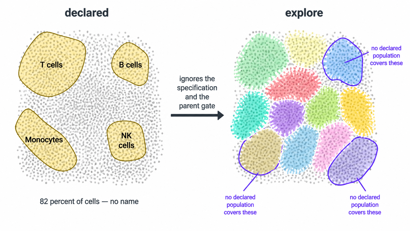
With --maybe-learn, this module has things a standalone clusterer does not:

From the declared run	What explore does with it
The transform, cofactor estimated on this panel	Clusters on the same scale the gates were drawn on, instead of an assumed default
A threshold for every marker in every sample	Names each cluster from the fraction of its cells above that sample’s own cut
Staining QC verdicts	Records them per cell, without excluding. See section 5
The batch/group confounding verdict	Carries it into the cluster statistics, so a q-value cannot be read without it

The result is a phenotype with a measurement behind it: CD19+ HLA-DR+ CD3- CD14-, where every call is a percentage of cells above their own sample’s threshold, rather than a colour you interpreted.

Run without --maybe-learn, explore is blind: it sees the transform and the group labels and nothing else. It names its clusters against cuts it places on each sample’s own cells by the declared run’s rule (a valley, else a tail gate above the dominant mode), reading none of the declared run’s cuts, and calls a cluster debris when most of its cells sit below its file’s CD45 debris reference, the 99.5th percentile of CD45 on the events the scatter gate rejects, as the declared CD45 gate defines CD45-negative. A pooled median, used before for the names, calls half of all cells positive for every marker; a 2-means split of cluster medians, used before for debris, cut through CD45-dim cells on PBMC. Blind is the right default, and section 6 explains why.

2. The three ways to run it

Alongside the declared analysis

docker run --rm \
  -v "$PWD/data:/data:ro" \
  -v "$PWD/results:/results" \
  cyraven:1.0.0 \
  --dir /data/fcs \
  --samples /data/samples.csv \
  --config /data/panel.yaml \
  --group-column cohort \
  --reference-group "Healthy controls" \
  --cluster \
  --explore \
  --outdir /results

Both analyses run. The declared deliverables are byte-identical to a run without the flag; explore’s outputs are in results/explore/.

Alongside, and linked

  ... --explore --maybe-learn

The two inform each other, in both directions. See section 6.

Standalone, with no specification at all

docker run --rm \
  -v "$PWD/data:/data:ro" \
  -v "$PWD/results:/results" \
  cyraven:1.0.0 \
  --dir /data/fcs \
  --explore-only \
  --outdir /results

No --config, no --samples, no populations. Just a folder of FCS files. This is the mode for a panel you have not written a specification for yet, and explore_suggested_spec.yaml is where you get a first draft of one.

3. What it clusters on

Every eligible channel, including scatter and viability. No lineage preference, no exclusions. That is the unsupervised default and it is deliberate: it is what lets the QC gate find debris (CD45 low), dead cells (viability high) and granulocytes (side scatter high, identified by no antibody in most panels).

The cost: some clusters will split on scatter rather than on lineage. If that is not what you want:

# cluster on these markers only
--explore-markers CD3,CD4,CD8,CD19,CD56
# or drop the usual suspects
--explore-exclude FSC-A,SSC-A,LiveDead

4. The quality gate

cyRAVEN’s declared path starts by gating CD45-positive leukocytes. Explore mode cannot: a declared parent gate is exactly what it is meant to work without.

So it uses the cluster-level gate the unsupervised family uses. Cluster coarsely first, then judge whole clusters by their marker profile, so no per-event cutoff is invented. The units judged are the SOM nodes (100 on the default 10 × 10 grid), not the merged clusters: a merge can join debris to CD45-dim cells that border it, such as low-density granulocytes in PBMC, and whether it does depends on the seed. Node by node, the same rule keeps those cells at every seed.

Call	Rule
debris	Leukocyte marker low across the cluster
dead	Viability dye high across the cluster
saturated	Top percentile in most channels at once. No real cell type is, so these are aggregates and doublets

Saturation is decided first: an aggregate is bright in the leukocyte marker too, so calling it debris would mislabel it.

Under --maybe-learn the debris and dead calls are made against each sample’s own thresholds. Without it they come from 2-means on the per-node medians, which is what a standalone tool has. Either way explore_qc_clusters.csv records the call and the basis for it per node, with the merged cluster each node belongs to.

If the gate would keep less than --explore-min-retained (default 5%), it is ignored and the run flagged: at that point the markers are more likely mis-named than the data bad.

# embed every event, debris included
--no-explore-qc
# keep the cluster marked dead
--explore-keep-dead

5. Two things it does that the declared path cannot

It keeps the samples staining QC excluded. A sample with no resolvable CD45 mode has no usable parent gate, so the declared path must drop it: every percentage would be a fraction of an arbitrary slice. Explore does not depend on that gate, so those samples still contribute, and staining_qc_verdict is a column rather than a filter. On a cohort where three samples failed, that is three donors you can still say something about.

It looks outside the parent gate. Anything the CD45 gate excluded is invisible to the declared analysis by construction. Explore embeds it.

6. --maybe-learn, and why it is off by default

Without the flag the two analyses are computed in complete isolation. That is not caution for its own sake:

• An explore run that used the declared thresholds is no longer a blind unsupervised run. If you want to compare cyRAVEN’s clusters against another tool’s, or check whether the specification is any good, the check has to be independent of the thing being checked.
• A declared run carrying a diagnostic derived from clusters is no longer the run its manifest describes.

With the flag, both directions open:

Declared to explore. Per-sample thresholds name the clusters, QC verdicts are recorded, the confounding verdict is attached to the statistics, and the bridge tables against the declared populations are written.

Explore to declared. One file appears in the run directory: spec_gaps.csv, with two kinds of row.

issue	Meaning
population spans several clusters	The declared label lumps distinct phenotypes. Its total can be flat while a subset inside it moves
cluster no declared population covers	Something in the blood nobody declared

The first row type is the one worth the flag. A declared population whose total does not differ between groups, while a cluster inside it does, is invisible to any amount of testing on the declared table, and it is a real pattern, not a hypothetical.

7. What it writes

All in <outdir>/explore/.

File	Content
explore_report.html	Start here. Self-contained, every figure and table embedded
explore_cluster_profile.csv	Per cluster: size, phenotype string, fraction positive and median per channel
explore_qc_clusters.csv	The gate: call and basis per coarse cluster
explore_cluster_abundance.csv	Per donor per cluster, with counting uncertainty and LOD/LOQ
explore_cluster_stats.csv	Group tests, donor-level, with the confounding verdict attached
explore_cells.csv	One row per cell: sample, event index, cluster, UMAP coordinates
explore_vs_populations.csv	Cross-tab against the declared labels
explore_findings.csv	Clusters no declared population covers
explore_population_split.csv	Declared labels spanning several clusters
explore_suggested_spec.yaml	A draft specification, for curation
explore_provenance.csv	Every choice made, and on what basis

Figures: explore_umap_clusters.png, explore_cluster_heatmap.png, explore_umap_by_group.png, explore_umap_markers.png, and explore_marker_umaps_by_group/, one panel per group per marker, on the shared embedding.

The report is separate from report.html rather than a section inside it, for the reason in section 8: report.html is a declared deliverable and --explore must not change it.

What each cluster corresponds to, and what it is

Two questions, two answers, and they can disagree.

Correspondence is measured by which cells overlap. explore_cluster_identity.png puts clusters in rows and declared populations in columns, grouped by the population each cluster best matches. The match is scored by the F1 statistic, the harmonic mean of precision (how much of the cluster is that population) and recall (how much of that population is in the cluster), rather than by the largest overlap. The distinction matters: a cluster of 500 cells holding 300 CD4 T cells has CD4 as its plurality even when those 300 are a twentieth of the CD4 T cells in the run. The label would describe the cluster; the cluster would not describe the label. F1 can only be high when both directions hold. The method follows Weber & Robinson, Cytometry A 2016;89:1084-1096, who match clusters to manually gated populations this way.

Every cluster has a best match, so the call is qualified rather than asserted: confident at F1 ≥ 0.5, partial, or no clear match, all written to explore_cluster_identity.csv with the precision and recall behind them.

The catch-all is ranked apart, because it is the complement of the specification rather than a cell type. Letting it compete would name most clusters “Other” on a specification with modest coverage, which is true but not informative. A cluster at or above 70% catch-all is reported as undescribed, which is a gap in the specification rather than a property of the cluster. A cluster half or more catch-all is never called confident, however clean its F1 against the remainder.

Identity is read from the cluster’s own marker profile. explore_cluster_subsets.csv matches each cluster’s positivity fractions against the immune subsets the panel can express (activated, exhausted and homing T cell subsets, NK CD56 bright/dim, HLA-DR low and CD38+ monocytes, and so on) and takes the most specific definition the profile satisfies. The base lineages are candidates too, so a cluster of plain CD4 T cells is named rather than left blank. The margin column is the smallest distance from the positivity cut across the requirements that were checked: a cluster 51% positive for a marker satisfies the same requirement as one 99% positive, and only the margin separates them.

This is written whether or not a specification was scored, so an explore-only run still gets it.

The subsets a panel can define are a property of the panel, not of immunology. Only definitions whose every marker is present are proposed, and the canonical groups that cannot be reached are named in the log with the markers they would need: naive/central-memory/effector-memory without CD45RA and CCR7, the three monocyte subsets without CD16, senescent T cells without CD28.

The subsets are not added to the declared specification. Appending them there re-scores every cell, changes every frequency and legend, and asks a circular question of a subset named after the marker that defines it: a CD69+ subset is 100% CD69-positive by construction. The annotation attaches to the cluster, never to the cell, and no declared output changes.

The heatmap is fractions, not medians

explore_cluster_heatmap.png plots the fraction of each cluster positive for each marker, not the median expression. A median is a number on a transformed scale whose apparent meaning depends on the colour limits you chose. A fraction positive is “this share of the cluster is above its own sample’s cut”, which is the same quantity a person reads a gate for.

8. The isolation guarantee

--explore must not alter a single byte of the declared deliverables. That is tested rather than asserted: the demonstration cohort is run with and without the flag and every top-level output compared byte-for-byte, excluding only run_manifest.txt and report.html, which embed a timestamp.

The two new tables in section 9 are the one intended change, and they appear on every run, with or without explore.

spec_gaps.csv is the only file explore is ever allowed to add to the declared output, and only under --maybe-learn.

9. The statistics catalogue

Two files now appear in the normal output on every run, and they exist because a reader arriving from an immunophenotyping paper expects t-tests and ANOVA and finds rank tests instead.

statistical_methods.csv lists every commonly reported method: Student’s and Welch’s t, one-way and two-way ANOVA with Tukey, repeated measures, Mann-Whitney, Kruskal-Wallis with Dunn, chi-squared, Bonferroni, and the cytometry-specific diffcyt family (edgeR, limma-voom, GLMM), and for each one says whether this run computed it and why. The edgeR form runs with --edger.

normality_tests.csv carries the evidence: a Shapiro-Wilk test per population per group, and a Brown-Forsythe test for equal variances across groups. Those are the two assumptions a t-test or ANOVA rests on.

What it will usually show, and the reason the interpretation column exists: Shapiro-Wilk on 4 to 10 donors has almost no power, so a non-significant result is not evidence of normality. That is why the rank test is used, and the table says so rather than leaving a reader to conclude “p > 0.05, so a t-test would have been fine”.

What does not happen: running every test and reporting all the p-values. At these group sizes that is p-hacking with extra steps.

10. Options

Option	Default	Effect
--explore	off	Run explore alongside the declared analysis
--explore-only	off	Run only explore; no specification needed
--maybe-learn	off	Let the two analyses inform each other, both ways
--explore-k	20	Metaclusters
--explore-qc-k	20	Merged clusters of the coarse QC clustering; the gate judges their SOM nodes
--explore-grid	10	SOM grid side
--explore-neighbors	30	UMAP n_neighbors for the explore embedding
--explore-min-dist	0.1	UMAP min_dist for the explore embedding, separate from --min-dist (0.3)
--explore-cells-per-sample	6000	Cells drawn per sample before the gate
--explore-max-cells	150000	Ceiling across all samples
--explore-markers	every channel	Cluster on these only
--explore-exclude	none	Drop these channels
--no-explore-qc	off	Embed every single cell, dead and CD45-negative cells included
--explore-keep-dead	off	Keep the dead cluster
--no-explore-equalise	off	Keep every gated cell instead of equalising per sample
--explore-min-retained	0.05	Ignore the gate below this retention and flag the run
--no-explore-spec	off	Skip the draft specification

11. What explore mode is not

It is a hypothesis generator. A cluster is not a population until it has been declared, thresholded per sample, and checked.

The intended path is a loop: explore finds something to you curate explore_suggested_spec.yaml into a real specification to the supervised path scores it with per-sample thresholds, propagated uncertainty and the six specification checks to and if it survives, --explain-clusters and --export-gates turn it into gate geometry a sorter can be driven with.

Discovery is the beginning of that loop, not the end of it.

See also

• Running cyRAVEN: every command, and which to use when
• Diagnostics: the checks in reading order
• Statistics: why the donor is the unit of replication
• Interoperability: handing a cyCONDOR clustering to cyRAVEN

Diagnostics, in reading order

Population labels in cyRAVEN derive from a specification declared before the data were examined. That specification is a hypothesis about how the panel behaves across the batch, and it can fail in ways that a frequency table cannot express. The outputs below exist to detect those failures.

Sections 1 to 3 are sufficient to reject most compromised runs and should be read first. report.html presents all of them in this order, embedded in one self-contained file.

0. Before the run: --check

Every check below is applied to a run that has already happened. Some failures are knowable before it starts, from the FCS headers alone: a file the sample sheet has no row for, a specification naming markers the panel does not contain, a group column that does not exist or has one level, a subject whose rows disagree about that subject.

docker run --rm \
  -v "$PWD/data:/data:ro" \
  -v "$PWD/results:/results" \
  cyraven:1.0.0 \
  --dir /data/fcs \
  --samples /data/samples.csv \
  --config /data/analysis.yaml \
  --outdir /results \
  --check

It reads keyword blocks rather than events, so it costs seconds regardless of cohort size, and writes nothing. A marker name that does not match $PnS exactly is the most common cause of an empty frequency table, and it is the first thing --check reports.

Run it after every edit to either input file.

1. Gate inspection

recon_diagnostics.png and gating_qc.png are written unconditionally and show, per sample, the scatter gate boundary, the singlet band, and every marker threshold superimposed on the density from which it was derived.

A threshold placed on a distribution shoulder rather than a minimum is visible here and is not detectable in any downstream table.

1a. Acquisition stability

Every number reported for a sample is derived from that sample’s pooled events, which is correct only if the instrument behaved the same way throughout the acquisition. A partial clog, a bubble or a drift in laser power makes a file two instruments over its run, and one threshold then suits neither half.

acquisition_qc.csv bins the Time channel into equal-width intervals and tracks two quantities across them: the event rate, which a clog lowers and a bubble spikes, and each channel’s median, which catches a shift the rate does not show. Bins are equal in time rather than in count, because a bin holding a fixed number of events cannot reveal that the rate changed. acquisition_qc.png draws the rate per sample with the flagged intervals marked, and acquisition_qc_bins.csv holds the per-interval detail.

Nothing is removed. acquisition_qc_impact.csv states how far each population would move if the flagged intervals were excluded, and that is the number the decision rests on: a file with a visible anomaly that moves no population by more than its own gate uncertainty does not need re-acquiring. Compare pct_delta_if_cleaned against u_pct_points for the same population before concluding anything. --drop-unstable-events performs the exclusion and is recorded in the manifest.

A file carrying no Time channel is reported as such rather than as stable.

1b. Why a threshold did not resolve

Section 1 shows that a marker had no density minimum and got a tail gate. spreading_receivers.csv and spreading_pairs.csv are what distinguish the two reasons it can have.

Compensation removes the mean contribution of one fluorochrome to another detector. It cannot remove the photon-counting variance that came with it, so a receiver channel’s negative population is wider wherever a spilling source is bright. A widened negative fills the density valley a threshold would sit in, and no gating strategy recovers a minimum that the optics erased.

spreading_pairs.csv reports, for every ordered source and receiver pair, the ratio of the receiver’s negative spread when the source is bright to its spread when the source is dim. spreading_receivers.csv ranks receivers by their worst source and pairs that against how often the marker had no density minimum (fallback_rate, tail gates and quantiles together).

Read the two columns together. A marker with a high fallback rate and substantial spreading is failing for a panel design reason, and the fix is a different fluorochrome assignment rather than a different threshold method. A marker with a high fallback rate and no spreading is failing for some other reason: too few positive events, a titration problem, or a continuous distribution. Reporting the fallback rate alone cannot tell those apart.

2. Staining QC

staining_qc.csv records a per-sample verdict. A sample with no resolvable CD45⁺ mode contains no usable parent gate; it is excluded and the exclusion reported, rather than contributing a spurious frequency to a group mean. Samples declared as controls through the is_control column of the sample map are excluded from testing without being recorded as failures.

--include-qc-failed overrides exclusion for inspection.

3. Phenotype concordance

population_marker_heatmap.png displays marker intensity against declared populations, z-scored across the run.

In clustering-first analysis this figure assigns identity. Here identity is already declared, so the figure serves the inverse function: a column labelled CD4 T cells that does not show elevated CD4 and depressed CD8 falsifies the gate that produced it. The figure outlines the markers each population’s specification requires to be positive, reading the same populations: block used for scoring, so the audit cannot diverge from the definitions being audited.

cohort_composition_heatmap.png normalises each group to a common notional cell count before partitioning by population, which prevents unequal sample numbers or acquisition depth from generating the pattern.

4. Threshold drift

Per-sample thresholding introduces a specific hazard. If thresholds for a given marker differ systematically between study groups, the populations defined by that marker are not identically specified across the comparison, and any abundance difference is partly definitional.

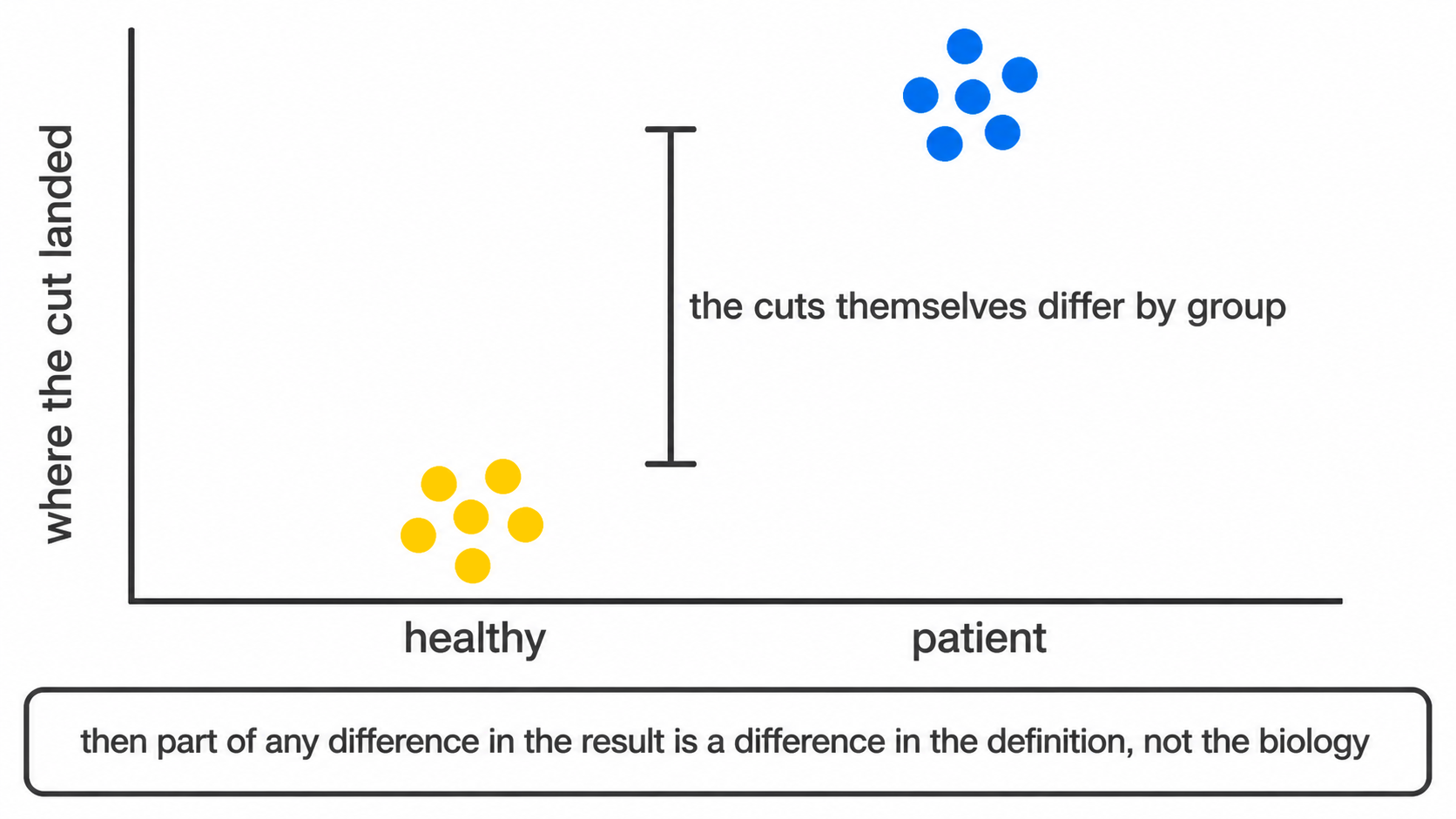
threshold_drift_stats.csv tests each marker’s per-sample thresholds against group membership and flags those that separate. A flagged marker invalidates naive interpretation of every population depending on it.

No clustering-based method has an equivalent output, because none carries a prior definition capable of drifting.

5. Gate uncertainty

Threshold drift asks whether a cut sits in a different place for one group than another. This asks a prior question: how well is it determined at all.

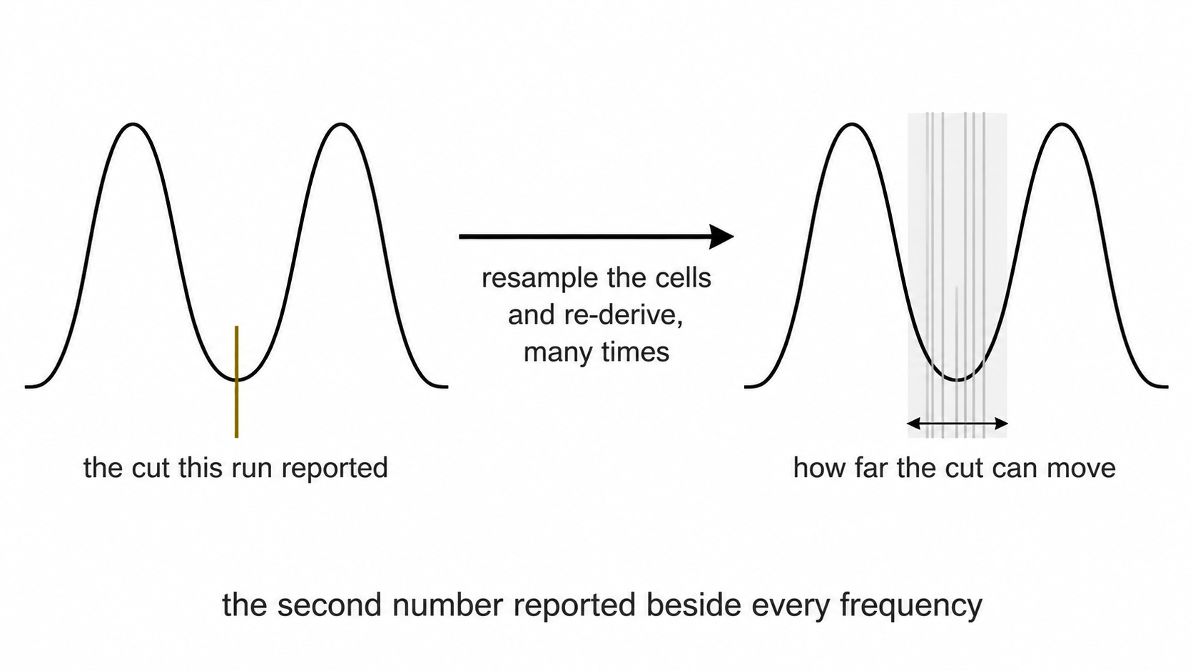
Each cut is re-derived from resamples of the events it was computed on, and again across the settings that placed it, and the two spreads combine in quadrature following the GUM convention. threshold_uncertainty.csv reports both components. uncertainty_budget.csv propagates them to each population, with the CD45 parent gate as a term in every one, since it fixes the denominator all frequencies are expressed against.

Read bootstrap_valley_rate before u_combined. A cut recovered in every resample is a population boundary. One recovered in half of them is histogram noise that happened to clear the depth rule, and the two are written to thresholds_used.csv in exactly the same way.

frequency_uncertainty.png places the two quantities side by side: the spread between samples, and the bar within each. Where the bars are as wide as the scatter, the variation on display is the cut moving rather than the biology, and difference_over_gate_u in the group comparison states the same thing for a tested difference. Below one, the groups differ by less than the distance the threshold itself travels under resampling.

The published figures for manual gating are the comparison worth making. Operator studies following the same convention report expanded uncertainty rising from around 12% on a three-gate strategy to around 16% on a five-gate one, with the first gate contributing most of it (Grant et al. 2021, Methods Protoc 4:24).

5a. Detection limits

The preceding section asks how well the cut is determined. This asks whether enough cells were counted for the answer to mean anything, which is a separate question with a separate failure mode: a cut through a wide empty gap is well determined however few events lie beyond it.

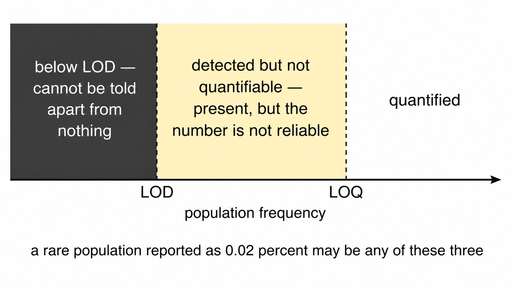
u_counting_pct_points in population_frequencies.csv is the uncertainty the frequency carries from its own event count, and u_total_pct_points combines it with the gate term. difference_over_total_u in the group comparison applies the same reading as difference_over_gate_u against both components and is the stricter of the two; the two separate exactly where a well-placed cut sits in front of too few cells.

detection classifies each value against the conventional twenty and fifty events, expressed as lod_pct and loq_pct of that sample’s parent gate.

detection_limits.png counts how many samples clear each limit, per population. Three readings:

A population quantified in every sample is measurable in this cohort.

A population mostly below the limit of quantification is not, and the gating strategy is not the reason. The numerator is small because few cells were acquired, so the remedies are a longer acquisition or a higher --max-events-per-file, not a different threshold.

A population split across the limit is the case to be careful with, because a group difference in it can be produced entirely by which samples happened to clear the limit.

Both limits are computed against the parent-gate events this run saw, so subsampling raises them proportionally. That is deliberate: it reports the resolution of the analysis that was actually performed rather than of the files on disk.

6. Cluster concordance

--cluster computes a self-organising map clustering of the same cells without reference to the specification, then cross-tabulates. Four configurations are diagnostic.

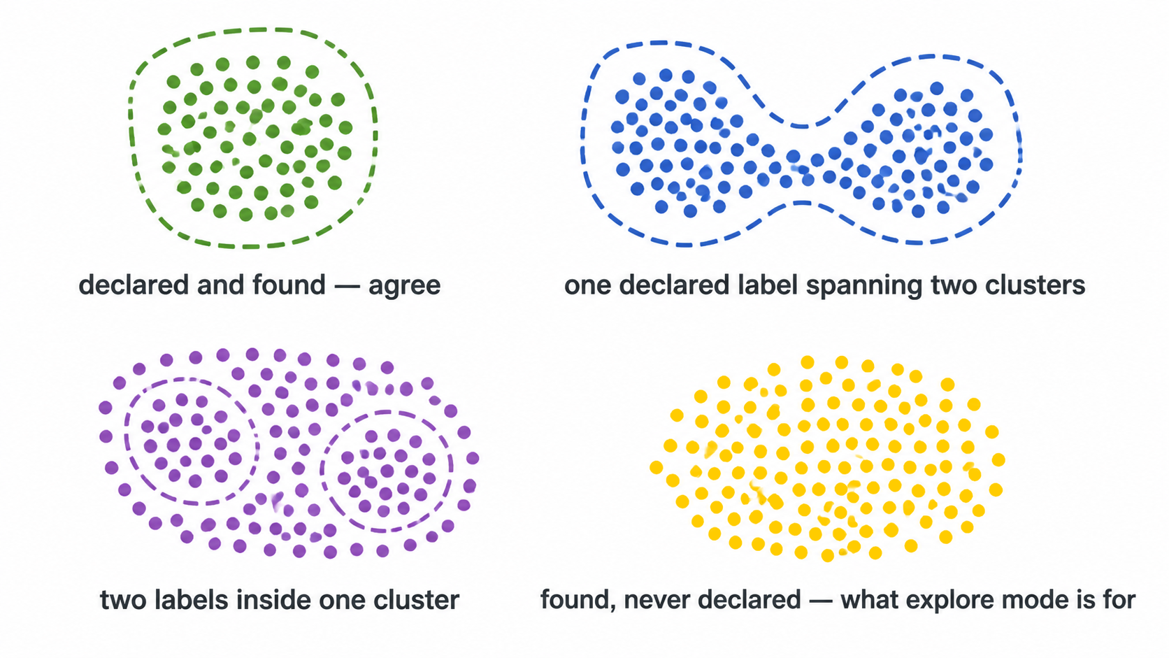
This check clusters WITHIN the parent gate, on the cells the specification already selected. --explore is the wider version: it clusters the single cells of the file over every eligible channel, so it can also find a population the CD45 or viability gate excluded. Under --maybe-learn it writes spec_gaps.csv, which names declared populations that turn out to span several clusters. See Explore mode.

6.1 Concordant. A cluster composed predominantly of one declared label. The specification and the data agree.

6.2 Undescribed population. A cluster dominated by the unassigned label. A phenotypically coherent population exists that the specification does not describe. Supervised analysis cannot produce this finding, since it has no mechanism for detecting an entity it never declared.

6.3 Under-specified label. One declared label distributed across several clusters. The definition is coarser than the phenotypic structure. Where the constituent subsets respond in opposite directions, the aggregate frequency reports no change.

6.4 Misplaced threshold. A label containing substantially fewer cells than the cluster it dominates. If CD4 T cells score 0.3% while a cluster comprising 20% of events is CD4-bright and unassigned, the population is present and the Boolean rule is rejecting it. This is the diagnosis a frequency table structurally cannot deliver.

Output: cluster_gate_agreement_clusters.csv, cluster_gate_agreement_populations.csv.

7. Gate transferability

A gate fitted to one cohort is worth having only if it selects the same population in the next one. --external-labels takes a cell labelling produced elsewhere, a cyCONDOR clustering for instance, learns a strategy for it, and then withholds one donor at a time: the whole strategy is refitted on the remaining donors and scored on the donor that was held back.

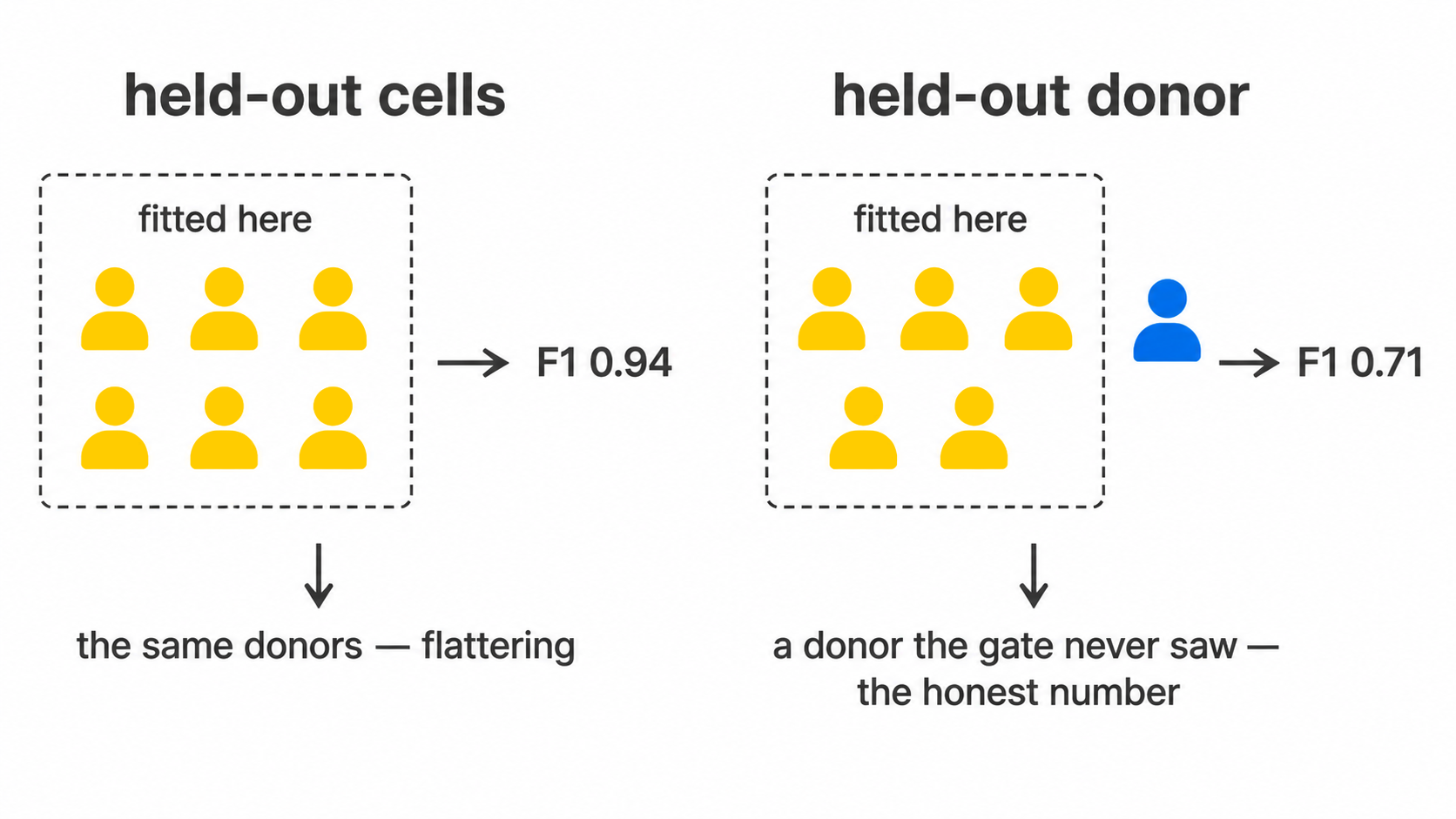
This is a different measurement from the held-out metric in section 8. Cells reserved from a fit come from the same donors, acquired in the same tubes on the same day, so they share every source of between-donor variation the gate will meet in use. A strategy can score an excellent held-out F1 on cells and still fail on the next patient.

gate_transferability_summary.csv reports the minimum, median, maximum and IQR across donors. Read the minimum. A gate scoring 0.9 on every donor and a gate scoring 1.0 on nine donors and 0.1 on one share a median and are not the same gate.

The join between the label file and this run is on sample and event index rather than row position, because two tools subsample independently and a positional join relabels every cell without raising anything. join_external_labels() reports the matched fraction and declines below a hundred cells.

Output: external_label_gates.csv, gate_transferability.csv, gate_transferability_summary.csv, and with --export-gates, a Gating-ML 2.0 document in the linear units the FCS file stores.

8. Gate geometry

A cluster index and a cell count are not actionable at the instrument. --explain-clusters converts an undescribed cluster into executable gate geometry.

For each qualifying cluster, cyRAVEN selects the two most discriminating markers, fits a convex polygon in that plane, retains the enclosed events, and recurses. The output is the topology of a manual gating strategy and can be reproduced by hand.

Convex polygons rather than rectangles: a conjunction of one-dimensional thresholds is an axis-aligned rectangle, and CD4 against CD8, CD14 against CD16, and FSC-A against FSC-H all separate along oblique boundaries. A rectangle imposed on an oblique boundary must either admit contaminating events or exclude genuine ones. derive_singlet_band() is a hand-written instance of the same geometry.

Every reported metric is computed on events held out of the fit, with the resubstitution value printed alongside. Eight free half-planes can memorise a few thousand events, so the difference between the two quantifies overfitting.

The stage is descriptive. A proposed gate localises events in marker space without asserting that they constitute a biological population. It carries no p-value, and scored frequencies and test results are identical whether it runs or not.

Output: cluster_gate_proposals.csv, cluster_gate_polygons.csv, cluster_gate_strategy_<k>.png.

9. Covariates

A variable confounds a comparison only when it both differs between groups and associates with the outcome within the groups. Either condition alone is inert, and flagging either alone would raise an alarm on any study with unequal age distributions.

confounding_diagnostics.csv reports both conditions using tests estimable at small n, and assigns a confounder_risk verdict. The outcome association is a partial Spearman correlation with the group held fixed (a rank F test for a categorical covariate): tested across the pooled groups, a real group difference makes any unbalanced covariate track the outcome by itself.

Adjustment is opt-in and kept separate. At single-digit n per group, a model carrying group with age and sex expends most residual degrees of freedom on nuisance terms. Where age is strongly associated with group, as in a syndrome-against-adult-control design, the parameters are not separable at any sample size: there are no young controls from which the age effect can be estimated independently. The adjusted estimate extrapolates beyond the observed covariate range and reports a confidence interval that does not reflect this.

--rank-ancova fits a rank-based ANCOVA where residual degrees of freedom permit, labelling every row EXPLORATORY. Where they do not, the output records NOT FITTED with the reason rather than a value that would appear comparable to the others in the folder.

9a. Clinical variables, which are the opposite question

--covariates names variables screened as nuisances: the question is whether a group difference can be believed in spite of them. --clinical-columns names variables that are the question: a severity score, a laboratory value, an outcome flag. Each is associated with every population and every marker. The same column would be a different analysis under each flag, which is why they are two flags.

One diagnostic belongs here rather than with the results. clinical_variables_correlation.png reports the clinical variables against each other, and is read before the association heatmap. p-values there are adjusted within each variable on the grounds that each variable is a separate question; in a cohort where the sickest patients are also the ones who died, SOFA and 28-day survival describe one gradient, and a population associated with both is one finding counted twice. No correction repairs that, and nothing else in the run would show it.

Read the effect and its bootstrap interval before the asterisk. At the sample sizes these designs have, an interval spanning zero is the usual outcome and is the informative part; underpowered marks every test run on fewer than ten samples, where a null result carries almost no information.

10. Batch structure

--batch-column names the variable identifying acquisition batch. Absent that, the $DATE keyword is used where it varies.

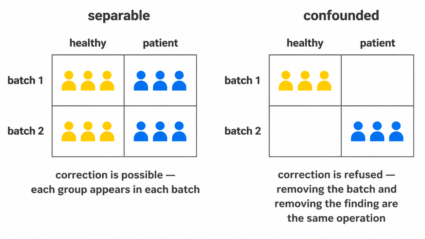
Two quantities are reported and both are required.

10.1 Magnitude. batch_mixing_stats.csv reports iLISI, the metric against which Harmony is evaluated, together with a permutation null. The null is necessary because the attainable score depends on the number and relative sizes of the batches, so an absolute iLISI is uninterpretable. Permuting batch labels and recomputing yields the score this dataset would produce under no batch structure.

10.2 Separability. batch_group_confounding.csv reports Cramér’s V between batch and study group, and between batch and timepoint where the sheet has one. Where patients and controls were acquired in distinct periods, V approaches unity and batch is not distinguishable from the comparison of interest.

10.3 Which channel. The two quantities above are properties of the shared embedding. Neither identifies the marker responsible, and a flagged embedding does not correspond to any action at the bench.

marker_batch_drift.csv compares each marker’s distribution between batches by Earth Mover’s distance, the L1 distance between their empirical quantile functions. It is reported in analysis units as emd_max, and divided by the marker’s own pooled MAD as emd_over_mad, which is the comparable form: a marker displaced by half its own spread is flagged regardless of the scale it sits on. worst_pair names the two batches responsible.

threshold_batch_drift.csv is the test in section 4 with batch substituted for study group. The two answer different questions and both are needed. A threshold is one number per sample, so it registers only drift that moves the cut; a marker can change its spread, grow a tail, or lose the separation between its modes while the density minimum between them stays exactly where it was. The distributional comparison sees that, and the threshold comparison cannot.

A marker flagged in either is a statement about the assay rather than about the donors, unless batch and study group coincide, which is what 10.2 establishes and should be read first. Where V is high, neither table separates a reagent lot from the biology.

Correction proceeds only when both readings permit it. --correct-batch aligns each marker across batches by monotone quantile mapping; monotonicity guarantees that within-batch cell ordering is preserved, so location and scale are adjusted without introducing structure. Above --batch-max-cramers-v correction is refused, since at that level of confounding removing the batch effect and removing the biological effect are the same operation. The default threshold is Cohen’s large association, w = 0.5, which is V = 0.5 for a two-level table and smaller for larger ones (0.35 for three levels). --force-batch-correction overrides, and the override is recorded in the run manifest.

--batch-method selects how the alignment is fitted, and is read only after the refusal has been evaluated, so both methods are refused on identical evidence. A better alignment algorithm does not make a confounded design correctable.

quantile, the default, fits one map per marker over the whole file. That is correct only when the batch effect is the same for every cell, which it often is not: a shift in a detector moves a bright population and a dim one by different amounts, so one map fitted to the pooled distribution over-corrects one and under-corrects the other. A per-file map also moves with the biology, so it can remove the difference it was meant to preserve.

cluster fits one map per marker per cell type, which is the published remedy and the method CytoNorm implements. Two stages, and the second is not optional: clustering the raw matrix lets a large batch shift become the dominant source of variance, so the clusters turn out to be the batches, each holding one batch with nothing to align against. The clustering is fitted on a whole-file-aligned copy and the per-cluster maps on the original values. Measured on a synthetic three-batch shift, the naive form left a mean between-batch gap of 1.296 against whole-file alignment’s 0.003; fitted correctly it reaches 0.014 while leaving the true between-cell-type separation at 3.996 against a true 3.994, where whole-file alignment inflates it to 4.078. cytonorm is accepted for cluster, with a note in the log: it is not the CytoNorm package, which learns its maps from anchor samples.

The goal each batch is aligned towards. Quantile alignment maps each batch onto a goal distribution. A goal pooled over every cell weights the batches by their cell counts and blends the study groups, so where one batch holds mostly patients and another mostly controls, aligning both to it pulls the groups together. Each study group is therefore aligned on its own, towards the mean of its batches’ quantiles, which is CytoNorm’s goal (Van Gassen et al. 2020) tailored to the design as CytoNorm 2.0 recommends (Quintelier et al. 2025). On a planted two-batch, two-group example the pooled goal shrank a 2-unit group difference to 1.2; the per-group goal kept 2.0 and removed the batch shift. --batch-pooled-goal restores the pooled form.

The clustering reuses the same seeded, stream-safe routine the unsupervised cross-check uses, so no dependency is added and a run reproduces. batch_correction.csv records which method ran, what it was judged on, and why, including when correction was refused.

Correction is applied to the shared embedding, the clustering and the gate-cluster concordance. It is not applied to per-sample frequencies, marker medians or the differential tests, which derive from per-sample thresholds and are batch-local by construction. The quantity a batch effect distorts is the single embedding computed across all samples.

11. Conformance

Every check above is internal to one run. This one is not.

The scale check (scale_outlier in thresholds_used.csv, summarised in threshold_scale_qc.csv) compares each threshold against the other samples of the same panel, which identifies a single deviant tube. It cannot identify a cohort that moved as a whole, because the leave-one-out peer median moves with it. After a laser service, a reagent lot change or six months of drift, every sample can agree with its peers and disagree with the assay as it was validated.

--write-baseline records where an accepted run placed each threshold, how variable it was, how often it needed the quantile fallback, and what the populations came out at. --baseline measures a later run against that record and writes specification_conformance.csv with a verdict per marker and per population.

The baseline holds summaries and the specification text, no event-level or patient data, so it belongs in version control beside the config it describes.

A failure is not a statement that the run is bad. It says the two runs no longer place their cuts in the same place, so their frequencies are not the same measurement and should not be pooled until someone has looked. --fail-on-drift turns that verdict into an exit code for scheduled runs, raised after every output has been written.

Cuts are compared in instrument units: each marker’s median cut is carried back through this run’s transform and forward through the baseline’s, because the cofactor and logicle widths are re-derived from every run’s data and a changed ruler would otherwise read as drift. Two results are withdrawn rather than reported: a cut whose transform cannot be rebuilt on both sides when the transforms differ, and a redefined population, which is a different population; both read not comparable, which is not a small drift.

12. Provenance

run_manifest.txt records the R version, platform, the version of every package loaded at run time, the git commit and working-tree state where the code was a checkout, the full invocation, and every option in force. It is written before the expensive stages and rewritten at completion, so an interrupted run leaves status: failed rather than an absent or misleading record.

miflowcyt.md restates the same run against the ISAC reporting checklist, which several journals check at submission. Its instrument section is read from the FCS keyword block: cytometer, serial number, acquisition software, date, operator and event counts per file, and per panel a detector table giving $PnN, $PnS, voltage, range and whether amplification was linear or logarithmic. Its data-analysis section is read from the run, so it cannot disagree with what was computed.

The two sections a run cannot establish, why the experiment was done and what the cells and reagents were, are marked TO BE COMPLETED. An omitted section reads as one that did not apply. Individual keywords follow the same rule and are reported as not recorded in the FCS file rather than dropped, since a missing $PnV or $SPILLOVER is usually the explanation for something further down.

--no-miflowcyt skips it.

Every output file

Reference for every file a run writes, its columns, and the flag that produces it. Worked examples of the principal figures, rendered from a run on public data, are in the Worked example; this article is the exhaustive list rather than a second copy of them.

1. Quality control

File	Content
recon_diagnostics.png	Gate boundaries per sample
gating_qc.png	Thresholds superimposed on the densities they derive from
staining_qc.csv	Per-sample verdict and exclusion reason, the CD45+ share of live cells and the live share of single cells (pct_live_of_singlets, empty where no viability gate was applied); pct_live_if_dominant_dead is the share below a dye minimum lying under the dominant mode, the live share if that mode is the dead cells (or empty), for a mostly dead sample the gate reads as mostly live; a second live mode near zero, common on whole blood, also produces one, so read it with the dye’s plot
margin_events.csv	Per file: margin events removed (or capped), events below a channel’s lower limit by flowAI’s rule (counted, not removed: in compensated data they are mostly cells bright in a spilling channel, and removing them would bias those cells’ frequency), channels linearised from $PnE, and the compensation applied
thresholds_used.csv	Threshold, derivation, cofactor and outlier status per sample and marker
thresholds_within_parents.csv	Cuts a population with parent: derives on its parent’s events, beside the CD45+ cut
threshold_scale_qc.csv	Per panel and marker: median, range, and how many cuts are scale outliers or fallbacks. Written when any cut is an outlier; the per-sample robust z is in thresholds_used.csv
acquisition_qc.csv, .png	Per-sample acquisition stability, and the flagged intervals
acquisition_qc_bins.csv	Per-interval rate and channel departure
acquisition_qc_impact.csv	How far each population would move if the flagged intervals were excluded
peacoqc_summary.csv	Per file, the events PeacoQC removed, the share each of its checks flagged, and a note where the isolation tree was not run (fewer than 150 time bins), written by --peacoqc
fmo_agreement.csv	Derived cut against its FMO-anchored equivalent, in units of the cut’s own uncertainty
controls_refused.csv	Channels where a declared control could not anchor a cut, and why
spreading_pairs.csv	Per channel pair, how much wider the receiver’s negatives become, overall and at a given source level, and trend_rho, a screen for compensation or unmixing error (trend_unresolved where spreading alone could produce the trend)
spillover_spreading_matrix.csv	The published spillover spreading matrix, written by --single-stains
spreading_receivers.csv	Per marker, total spreading received and whether it explains a fallback
calibration.csv	Bead fit per channel, written by --calibration-beads

thresholds_used.csv gains override_reason and override_by only when the config declares a sample_overrides: block, so a run that overrides nothing writes the table it always wrote. source is manual for an overridden cut, fmo_q995 for one anchored to a fluorescence-minus-one control, fmm_q995 for a tube that leaves out several reagents at once, and control_q995 for an unstained tube. Those three bare names mean the data indicated no cut (no density minimum: the tail gate or quantile it would otherwise have used is in derived_source) and the control supplied one; the _valley_rejected suffix means the data did indicate a cut and the control put the boundary higher, and fmo_q995_valley_lowered, under --fmo-sets-cut only, that a true FMO put it lower. Either way the row carries derived_threshold and derived_source, the cut that would have been used without the control, so the two stay comparable.

Only the FMO is a full reference. An unstained tube and a minus-multiple tube both lack the spreading the stained panel puts into a channel, so their negatives are narrower than the sample’s and the cuts they anchor are permissive on any channel that receives spreading (Roederer 2001; Maecker & Trotter 2006). spreading_receivers.csv names those channels; they are the ones worth an FMO.

What a control has to be before it is used

Two things go wrong with a control-anchored cut, so each declared control channel is checked before it is trusted.

A far quantile finds the edge of the negative population only when the control contains nothing but that population. A tube carrying roughly one percent of bright events puts the 99.5th percentile inside that tail instead. On the minus-multiple data this check was written against, one channel’s control sat at 1.0 at the 95th percentile and 5.6 at the 99.5th: a cut there was above the full stain’s own 99th percentile, so nothing in any sample would have been positive. The run also places the cut by the negative mode and the spread of the half below it, which a bright tail cannot move, and takes whichever of the two is lower. For a clean control that is the quantile, so nothing changes.

A minus control must also be dimmer in the channel it leaves out. When it is brighter, the tube, the sample sheet or the unmixing is wrong, and anchoring to it raises the cut and deletes a real population. Comparing the two negative modes in units of the sample’s own spread catches that. A refused control is listed in controls_refused.csv with its reason, and the threshold comes from the sample’s own data as it would have without any control.

Keep one consequence in mind when reading fmo_agreement.csv. A cut the control supplied has no uncertainty of its own, because the events behind it are in a different tube, so those rows carry distance but leave distance_in_u empty. The verdict scaled by uncertainty is therefore available for the rows where the sample’s own cut was the one applied, which are also the rows where the two methods were free to disagree.

Read acquisition_qc_impact.csv against u_pct_points for the same population before acting on an acquisition flag. --drop-unstable-events performs the exclusion; without it nothing is removed.

These constrain the interpretation of every subsequent file. A run whose gates are misplaced produces internally consistent statistics that are unusable.

2. Uncertainty

File	Content
threshold_uncertainty.csv	Sampling and method components per sample and marker, their quadrature sum, the valley’s relative depth, and the fraction of resamples that found it
uncertainty_budget.csv	Contribution of each threshold to each population’s uncertainty, per sample
frequency_uncertainty.png	Per-sample frequencies with their uncertainty, one row per population
uncertainty_budget.png	The same budget as a stacked median contribution
detection_limits.png	Samples per population, split by whether the event count clears each limit

bootstrap_valley_rate is the column to read first. A threshold found in every resample is a population boundary; one found in half of them is histogram noise that happened to clear the depth rule, and the two are indistinguishable in thresholds_used.csv.

u_combined is NA rather than zero where it could not be computed, which happens for a threshold taken from a separate control tube. u_n_terms_missing on the frequency table counts how many of a population’s markers contributed nothing, so a small total that is small only because most terms are absent is distinguishable from a tight one.

Two uncertainties are reported per frequency and they answer different questions. u_pct_points is placement: how far the number moves when the cuts behind it move. u_counting_pct_points is sufficiency: what it carries from the number of events counted, as the Wilson half-width at one standard deviation. u_total_pct_points is their quadrature sum. The two are alike for an abundant population and diverge for a rare one, where a cut through a wide gap is well determined and the count behind it is not.

lod_pct and loq_pct place the conventional twenty and fifty events on the percentage scale of that sample’s parent gate, and detection says which side of them the value falls. Both are set by what was acquired rather than by the gating strategy, so --max-events-per-file raises them in proportion; --lod-events and --loq-events change the conventions themselves.

Counting is not a row in uncertainty_budget.csv. That table answers which threshold a population’s uncertainty comes from, and counting is not a threshold.

Written by default. --no-uncertainty skips it and restores the previous output exactly.

3. Conformance

Written by --baseline.

File	Content
specification_conformance.csv	Per marker: this run’s threshold against the baseline’s, scaled by the baseline’s own spread, with a verdict
specification_conformance_populations.csv	The same for population frequencies
specification_changes.csv	Populations added, removed or redefined since the baseline

Three verdicts. pass is within tolerance, qualify is a marker worth looking at before pooling the two runs, fail says the cuts are no longer in the same place and the frequencies are not the same measurement.

not comparable is a fourth value and means the comparison was withdrawn rather than made: the transform differs from the baseline’s, so thresholds are on different scales, or the population was redefined, so it is a different population and a drift statistic would be a category error.

--write-baseline writes the reference itself. It contains summaries and the specification text, no event-level or patient data, so it can be version-controlled beside the config it describes.

4. Abundance

File	Content
population_frequencies.csv	Percentage of parent per population per sample
population_marker_mfi.csv	Per sample, population and marker: the median intensity on the analysis scale (median_asinh, which keeps its name under --transform logicle and holds the logicle value there), the same median in instrument units (mfi), and the percent positive
population_mfi_summary.csv	Median fluorescence intensity per population and marker: the median over donors of each sample’s median, in instrument units with its interquartile range, overall and per study group, with the median percent positive
population_composition.csv	Each population’s share of the embedded cells, its defining markers, its spread across donors, its share within each study group (pct_<group>, summing to 100 down each group), the same cells as a share of all embedded cells (pct_of_embedded_<group>, summing across a row to the population’s share), and the percent of it positive for each marker (pct_pos_<marker>)
population_composition_by_timepoint.csv	The same table for each timepoint, in the pooled table’s row order
functional_markers.csv	The same restricted to functional marker blocks declared in the config
population_ratios.csv	Derived ratios where declared
gate_counts.csv	Event counts at each level of the gate hierarchy
population_frequencies.png	Pooled composition across samples
population_marker_heatmap.png	Marker intensity against declared populations, z-scored
population_mfi_heatmap.png	MFI per population and marker, the value printed in each tile, colour scaled per marker; a bar per row gives the population’s share
population_mfi_dotplot.png	Dot size is the percent positive, colour the scaled MFI
population_mfi_heatmap_by_group.png	The MFI heatmap per study group, on one colour scale
umap_composition.png	The shared UMAP with a legend of each population’s defining markers, share of the embedded cells and that share split by study group with a total row, and a grid of the cells of each population positive for each marker. Every number is a percent of all embedded cells, so a row’s group columns sum to its share and no marker tile exceeds it
umap_composition_<timepoint>.png	The same figure for each visit, on the pooled map’s axes and in its row order

count is an event count and scales with acquisition duration. It is not an abundance. Report pct_of_cd45_pos unless absolute counts were supplied through --absolute-counts.

MFI is a median of medians, in instrument units. Each sample’s median comes first and the cohort value is the median of those, so donors are the replicates and the donor with the most events does not set the value. The median is taken on the analysis scale and inverted through the run’s transform; a median commutes with a monotone transform, so mfi is the median on the instrument’s linear scale exactly. Compare mfi between runs only when the instrument settings match: it is in the instrument’s units, which a voltage change rescales. The heatmap colours each marker separately, between its 1st and 99th percentile across populations, so the colour says “bright for this marker” and the printed number says how bright.

Composition shares sum to 100; frequencies do not. In population_composition.csv and umap_composition.png each embedded cell has one label, its most specific population, so “CD3 pos” holds only the CD3+ cells no deeper population claimed. population_frequencies.csv scores overlapping gates, where “CD3 pos” includes the CD4 and CD8 T cells. The shares are of the embedded cells, which are drawn per sample; pct_median_per_sample is the per-donor view. Under --subsample rare the shares are weighted back to the true composition.

5. Embedding

File	Content
cells_umap.csv	Per-cell coordinates with sample, population and panel
umap_overview.png	Embedding by population and by sample
umap_markers.png	One panel per marker
umap_density.png	Cell density in embedding space
umap_density_by_group.png	The same, faceted by study group
umap_overview_by_group.png	Combined embedding with one column per group
marker_umaps_by_group/	Full-size UMAPs per marker, in its own folder. umap_CD3.png pools every sample, and umap_CD3_by_<category>.png is written beside it for every category present, not only the --group-column one. Numeric columns, identifiers and single-level columns are not faceted; past four categories the extras are named in the log
umap_multigraph_overlay.png	Per-compartment marker distributions against the reference group
umap.model, umap.model.meta.rds	Persisted model, written by --save-umap-model

A persisted model permits projection of subsequent batches into the same coordinate space, holding cluster positions fixed between runs. Projection is refused where the new data lack markers the model used, since zero-filling would produce coordinates that are geometrically valid and biologically meaningless.

6. Inference

File	Content
group_comparison_stats.csv	Abundance between groups, per population
group_differences.png	Every population on one pair of axes: the effect against the evidence. The shortlist – read this to decide which panel below to read carefully
group_comparison.png	The same as per-sample distributions, one panel per population
marker_state_stats.csv	Differential state per population and marker
marker_state.png	The same as per-sample distributions
functional_markers_stats.csv	Functional blocks between groups
population_ratios_stats.csv	Declared ratios between groups
compositional_clr_stats.csv	Abundance tests on centred log-ratios
compositional_concordance.csv	Classification of each result against both parameterisations
edger_abundance_stats.csv	edgeR count-model test of each population’s cell counts, each group against the reference, written by --edger
paired_comparison_stats.csv	Paired designs, written by --paired-column
covariate_adjusted_stats.csv	Rank ANCOVA, written by --rank-ancova
subcluster_marker_shifts.csv	Pooled-event marker shifts per compartment
design_feasibility.csv	Which group comparisons can be made, and why the rest cannot
parametric_tests.csv	The t-test or ANOVA equivalent, with its assumptions recorded
posthoc_tests.csv	Pairwise comparisons by three methods, for three or more groups

Every file above except the last three uses one value per sample. subcluster_marker_shifts.csv operates on pooled events, carries effect sizes without p-values, and answers a different question from the tests above it.

group_differences.png

One point per population: Cliff’s delta on the x-axis, -log10 p on the y. A fold change of medians is the conventional x-axis and is the wrong one here, it is unbounded, and at single-digit group sizes it is decided by whichever sample sits at the median, so a population whose reference median is near zero produces a fold change of 40 that means nothing. Cliff’s delta is bounded [-1, 1], is the effect size the rank test corresponds to, and reads directly: 0.5 means the comparison group was higher in three quarters of the cross-sample pairs.

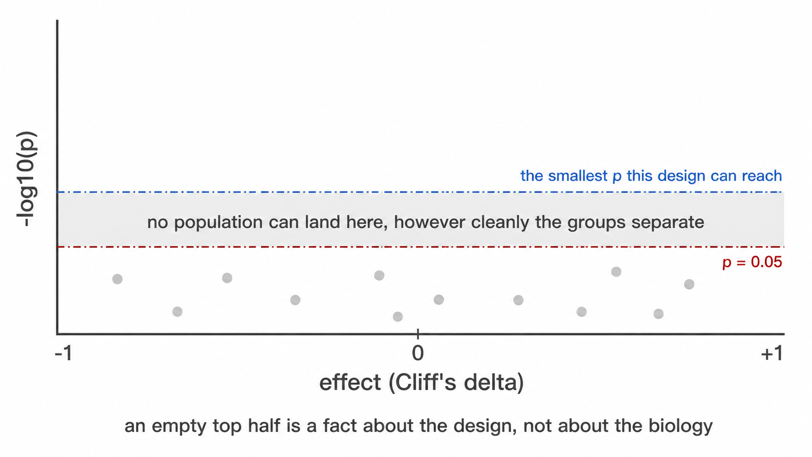
Two horizontal lines. The dashed red one is p = 0.05. The dot-dash blue one is the smallest p this design can produce at all: a Wilcoxon rank-sum test has choose(n1 + n2, n1) equally likely rank arrangements under the null, so the most extreme possible separation gives a two-sided p of 2 / choose(n1 + n2, n1) and nothing below it is reachable. At 4 against 5 that floor is 0.016, and after correcting across a dozen populations no population can reach 0.05 however cleanly the groups separate. When the blue line sits above the red one, an empty upper region of the figure says nothing about biology, it is a property of the design, and the figure says so rather than leaving the reader to work it out.

The floor is drawn per comparison, not once for the figure: each comparison group has its own size and so its own minimum, and 3 against 6 stops at 0.024 where 6 against 6 reaches 0.0022. With three or more groups the figure facets by comparison and each panel carries its own line.

design_feasibility.csv

Read before any of the tests. One row per group, carrying n_samples, n_donors, will_be_tested, valid_unpaired and a reason.

Two failures it is there to catch. A group smaller than --min-group-n is skipped, and a skipped comparison looks exactly like a comparison that ran and found nothing, because both produce no row. And a donor contributing to more than one group, which happens whenever the group column is a timepoint, makes an unpaired test treat repeated measures on one person as independent observations. That second one is the dangerous case, because the test runs and its output is well formed. will_be_tested says what the run did; valid_unpaired says whether it should have.

parametric_tests.csv and posthoc_tests.csv

The rank tests remain the primary result. These hold the parametric equivalents most immunology papers report, computed on the logit of each percentage (on log concentrations where the abundance is cells/µL), which stabilises the variance of proportion data. The transform column records which.

Two groups give Welch’s t-test with Student’s alongside it and Cohen’s d. Three or more give Welch’s ANOVA with the classical one-way alongside it and eta squared. posthoc_tests.csv then carries Games-Howell, Tukey HSD and Dunn for every pair. Their p_value differs in kind: Tukey HSD and Games-Howell refer to the studentized range and are already adjusted over the population’s pairs, Dunn’s is the unadjusted pairwise p (p_value_adjusted_over_pairs says which). p_adjusted_BH applies Benjamini-Hochberg within each test across every population and pair.

Every row records shapiro_p and brown_forsythe_p with the derived residuals_normal, equal_variance and assumptions_met. Where assumptions_met is FALSE the rank test is the defensible one, and the recommended column says which test to read. Normality is tested on the within-group residuals, not the pooled values, because pooled values are bimodal whenever the groups differ.

Disable with --no-parametric.

7. Diagnostics

File	Content
threshold_drift_stats.csv, threshold_drift.png	Whether thresholds separate by group
confounding_diagnostics.csv	Covariate imbalance, outcome association, and verdict
batch_mixing_stats.csv	iLISI against a permutation null
batch_group_confounding.csv	Cramér’s V and correction verdict
batch_diagnostic.png	Observed against null mixing
populations_by_batch.png	Every population’s abundance per acquisition batch, one box per batch and a point per sample. batch_diagnostic.png asks whether the embedding separates by batch; this asks whether the reported numbers do, which is the question that decides whether a group difference might be an acquisition difference

Clinical variables, written by --clinical-columns

A severity score, a laboratory value or an outcome flag is neither the study group nor a confounder. A confounder is screened to decide whether a group difference can be believed; a clinical variable is the question. Name any sheet column with --clinical-columns, or samples: clinical_columns: in the config , and it is associated with every population and every marker.

File	Content
clinical_variables_correlation.png	The clinical variables against each other. Read this first, see below
clinical_association.csv	One row per population × variable: test, n, the effect with its bootstrap interval, raw and BH-adjusted p, the levels or range tested, and an underpowered flag
clinical_association.png	Heatmap of the signed effect, populations against variables, with * on the tiles that survive correction
clinical_landscape.png	The whole cohort as one picture: one column per sample ordered by the first numeric variable, every clinical variable as a strip above, every population as a z-scored row below
clinical_effects_<variable>.png	Every population’s effect against that variable, ordered, with a 95% percentile bootstrap interval on each
clinical_<variable>.png	The data behind one column of the heatmap: a scatter against a numeric variable, a box plot against a categorical one, one point per sample and one panel per population. Where a categorical variable’s labels are too long to fit under the panels, such as organism names, each category gets a colour and is named once in a legend, with its sample count
clinical_association_markers.csv, clinical_association_markers.png	The same against each population’s median marker intensity, one test per population and marker (the pairs in functional_markers.csv)
population_trajectories.png	Written by --paired-column with --condition-column, and coloured by the first two-level clinical column when there is one: per-patient lines across the conditions with the median over them

The test follows the variable’s type rather than being chosen: Spearman’s rho for a numeric column, Wilcoxon rank-sum with Cliff’s delta for a two-level column, Kruskal-Wallis with epsilon-squared for more levels. Rank methods throughout, for the reason they are used everywhere else here, clinical scores are ordinal by construction, laboratory values are skewed with outliers that are real rather than erroneous, and cohorts are small.

Epsilon-squared is H / (n - 1), the proportion of rank variance the grouping accounts for. It is unsigned: a variable with three levels has a magnitude but no single direction, which is why the signed column exists and why those tiles stay grey on the heatmap rather than being coloured as though they pointed somewhere.

The effect, its interval, and why they come before the p-value

ci_low and ci_high are a 95% percentile bootstrap interval on the effect, 2000 resamples of the patient-value pairs for Spearman, stratified within each arm for Cliff’s delta, from a fixed seed so the same table always yields the same interval. clinical_effects_<variable>.png draws them ordered by effect.

On ten patients most intervals span zero, and that is the finding: a rho of 0.61 whose interval runs -0.1 to 0.9 is a lead worth powering a follow-up on, not a result. The interval is itself approximate at this size, below about nine observations the bootstrap’s effective resample is smaller than the nominal one and coverage falls short of 95%, so read a wide interval as this cohort does not constrain the effect rather than as a precise range. It is suppressed entirely below six samples rather than quoted at a width nobody should trust.

Read the variables against each other first

Benjamini-Hochberg is applied within each variable, which treats the variables as separate questions. That holds only when they carry different information. A cohort where the sickest patients are also the ones who died has one gradient and two columns describing it, and an association found against both is one finding reported twice. clinical_variables_correlation.png is where that is visible: circle area is the absolute Spearman coefficient, fill is its sign, and the number is printed where the unadjusted p-value is below 0.05. Two-level variables are included coded 0/1, for which Spearman is the point-biserial correlation of the ranks (not the rank-biserial: two perfectly separated groups of five give 0.87, not 1); variables with three or more unordered levels are excluded and named in the caption, because there is no ordering to correlate and coding them 1/2/3 would invent one.

Benjamini-Hochberg is applied within each variable, across the populations tested against it, because each variable is its own question asked of every population. Pooling across variables would penalise a well-powered variable for the company it keeps.

Two things this is not. It is not survival analysis: a 28-day flag is tested as the two-group comparison it is, and no time-to-event model is fitted because the sheet carries no follow-up time. And it is not a claim about cells: every test runs on one value per sample, so the replicates are subjects. Correlating a score against tens of thousands of events would treat one deeply acquired patient as tens of thousands of observations.

Read the effect before the asterisk. On a small cohort these tests detect only very large effects, so a null result says little, and the underpowered column marks every test run on fewer than ten samples. | marker_batch_drift.csv | Earth Mover’s distance between batches per marker, in analysis units and scaled by the marker’s own MAD | | threshold_batch_drift.csv | The threshold test above, grouped by batch instead of by study group | | batch_correction.csv | Whether a correction ran, which method fitted it, the Cramér’s V it was judged on, and the reason. Written whenever --correct-batch is set, including on a refusal |

The last two are written by --batch-column and answer the question the first three cannot: which channel moved. iLISI is a property of the embedding, so a flagged run names nothing actionable, whereas a flagged marker names a reagent lot or a detector.

Read emd_over_mad rather than emd_max: the raw distance is in the units of whichever marker it describes, and dividing by that marker’s own spread is what makes two of them comparable. worst_pair names the batches responsible.

Both tables are needed. A threshold is one number per sample and registers only drift that moves the cut, while a marker can change its spread or lose the separation between its modes with the density minimum between them unmoved.

File	Content
run_manifest.txt	Versions, commit, invocation, options

8. Clustering

Written under --cluster and --explain-clusters.

File	Content
unsupervised_clusters.csv, .png	Cluster assignment per cell
cluster_gate_agreement_clusters.csv	Dominant label and purity per cluster
cluster_gate_agreement_populations.csv	Recovery of each declared population
subcluster_k_selection.csv	Silhouette-selected k, from --auto-subcluster-k
cluster_gate_proposals.csv	Learned gate geometry with held-out metrics
cluster_gate_polygons.csv	Polygon vertices in transformed units
cluster_gate_strategy_<k>.png	One figure per explained cluster

9. External labels

Written by --external-labels, and by --export-gates for the last two.

File	Content
external_label_gates.csv	Learned strategy per supplied label, with held-out metrics at each depth
external_label_polygons.csv	Polygon vertices on the analysis scale
gate_transferability.csv	Precision, recall and F1 on each donor, from a strategy refitted without that donor
gate_transferability_summary.csv	Minimum, median, maximum and IQR of F1 across donors
external_label_strategy_<label>.png	One figure per label
*.gatingml.xml	ISAC Gating-ML 2.0, linear units, levels chained parent to child
*_polygons_linear.csv	The same vertices as a table, for redrawing by hand

Read f1_min from the summary, not f1_median. A gate scoring 0.9 on every donor and a gate scoring 1.0 on nine donors and 0.1 on one have the same median and are not the same gate.

The Gating-ML vertices are subdivided along each edge. An edge that is straight on the analysis scale is a curve in the linear units the FCS file stores, so a polygon built from the corners alone would describe a different region from the one that was fitted and validated. Dimensions are named by marker symbol, which is what cyRAVEN resolves from $PnS.

10. Auxiliary

File	Content
run_manifest.txt	R and package versions, git commit, invocation, options, run status
miflowcyt.md	The same run against the ISAC reporting checklist
report.html	Every output above embedded in one self-contained file, in the order this documentation says to read them. Written for failed runs too, with a diagnosis
patient_metadata_english.csv	Patient table after column mapping and value translation
absolute_counts.csv, absolute_counts.png	Measured cells per microlitre per sample and population, written by --absolute-counts
absolute_counts_raw.csv	The supplied workbook flattened to CSV exactly as read, before any header or population-name interpretation. Open this first when a population from --absolute-counts looks wrong: it separates a reading problem from a mapping one
absolute_counts_stats.csv	Between-group tests on the measured counts, on cells_per_ul. Written when the run performs group tests, so it needs --group-column and is absent under --no-group-tests
absolute_counts_qc.png	The supplied counts, one log-scale tile per sample and population, controls and QC failures labelled, same flag. Written unconditionally whenever counts are supplied, and deliberately before the group-comparison figure, because a unit or mapping error has to be visible before the more inviting figure is read as a finding
populations_unavailable.csv	One row per sample and population the panel cannot score, with the reason. Written only when there is at least one
flowjo/	UMAP-annotated FCS, written by --flowjo-export
config_derived.yaml	Derived parameters, written by --write-config
sample_map_template.csv	Written by --write-sample-map
gate_adjustments.csv	One row per hierarchy gate --auto-fix-gates skipped and per population cut it replaced, with threshold_not_applied, pct_of_parent_kept and the reason. Empty without the flag

Gate adjustments

Written only under --auto-fix-gates, and the one table to read before any frequency from a run that used it, because a skipped gate changes every count beneath it.

Column	Meaning
sample_id, gate, marker	Which cut, in which sample
threshold_source	Why it was eligible. quantile_fallback means no density minimum was found, so the cut came from a percentile
threshold_not_applied	The number that would have been used. Kept so the decision is auditable rather than merely reported
action	skipped, with the parent carried through unchanged; for a population cut, replaced by and the new value
pct_of_parent_kept	What the gate retains after the decision. 100 when it was skipped
reason	The rule that fired, in words

Two rules put a gate here. A threshold that came from quantile_fallback has its retention fixed by the fallback constant rather than by the data, so it keeps the same share of the parent whatever the sample holds. And a gate retaining less than 5% of its parent is misplaced whatever its source says, because a viability or CD45 gate that discards nineteen cells in twenty is not measuring what it claims to.

Population markers are never skipped: a quantile fallback on CD19 is a poor threshold, but “no threshold” does not mean “every cell is a B cell”. They borrow instead (--peer-cuts, which --auto-fix-gates implies). Every sample of a panel is on one pooled transform, so where most of them found a density minimum for the marker, the median of those minima is a measured cut on this sample’s scale too, and a sample without one – a quantile_fallback or a tail-rule cut – takes it. Where most samples found none, as for a rare marker, the tail rule stands, and only a fallback or a tail cut more than 3.5 robust SDs from the other samples’ cuts takes their median. The row in thresholds_used.csv then has source peer_median, keeps needs_review, and holds the original cut in derived_threshold. The same applies to the functional-block markers, whose positive fractions use these cuts. Cuts from a control, a config entry or a manual override are never replaced.

10d. Externally measured cell counts

Written by --total-counts. A share is constrained to sum to 100, so a frequency table cannot distinguish one population expanding from every other contracting. A measured yield per acquisition is what separates the two.

File	Content
total_counts.csv	The yields as parsed and matched: patient_raw, timepoint, total_cells, sample_id. One row per acquisition that matched
total_counts_raw.csv	The sheet flattened exactly as read, before any header or block interpretation. Open this first when a number looks wrong: it separates a reading problem from a matching one
total_counts_qc.png	Read this before anything derived from it. The yields on a log axis. Everything downstream inherits their error, and a yield in the wrong unit lands decades off the median here while staying invisible in the derived table
absolute_vs_share.png	The two measures side by side per population. Where a global depletion is visible as the thing a share cannot express
absolute_vs_share_by_timepoint.png	The same, once per visit, under --split-by-timepoint
explore_total_counts_qc.png, explore_absolute_vs_share.png	The twins of those two inside explore/
explore_cluster_stats_absolute.csv	Inside explore/: the donor-level cluster tests on cells per cluster, kept apart from the share tests in explore_cluster_stats.csv
explore_cluster_count_concordance.csv	Inside explore/: per cluster, whether the two agree. absolute only is a compartment that changed size with its composition unchanged; share only is a redistribution

population_frequencies.csv gains total_cells, cells_absolute and count_basis; where the sheet carries blood_volume_ml it gains cells_per_ml as well, which is the column to read across timepoints because the draws differ in volume.

count_basis records the route on every row that carries one. Treat cells_absolute as dual-platform: one measurement from this run multiplied by one from an instrument it never saw. Published interlaboratory CVs for that route are roughly 20-33%, against 10-16% for single-platform bead counting, so a difference smaller than that is unresolved. Shares are never overwritten.

10e. Clinical variables

Written by --clinical-columns. One figure per variable, plus the effects across populations.

File	Content
clinical_<variable>.png	One figure per variable named to the flag, showing the association with every population
clinical_effects_<variable>.png	The effect sizes for that variable with their bootstrap intervals, populations ordered by effect
clinical_association.csv	Every variable against every population: the test chosen from the column’s type, estimate, effect, ci_low, ci_high, p_value, p_adj_BH, and underpowered
clinical_association_markers.csv, .png	The same against marker expression within each population rather than abundance
clinical_variables_correlation.png	Read this first. p-values are adjusted within each variable on the assumption that the variables are separate questions, and this is where you see whether they are
clinical_landscape.png	Every clinical variable and population on one grid, columns ordered by timepoint then study group
clinical_timepoint.png, clinical_infection_focus.png	A categorical clinical column gets the same treatment as a numeric one, with the test following the type

n_patients and repeated_measures on every row say what the test actually had: a variable that is a property of the donor is tested at the donor level even when several acquisitions carry it, because the unit of replication is the donor.

10f. The figure set per visit

Written by --split-by-timepoint into by_timepoint/<level>/, plus the paired views that need every visit at once and so stay in the run directory.

File	Content
by_timepoint/<level>/	The whole figure set again, restricted to that visit
timepoint_trajectories_pct_of_cd45_pos.png	One line per patient across visits, on share
timepoint_trajectories_cells_absolute.png	The same on absolute cell number, with --total-counts
timepoint_trajectories_cells_per_ml.png	The same per millilitre, where blood_volume_ml is supplied. This is the one to read across visits, because the draws differ in volume
timepoint_subset_balance.png	Subset composition by visit
timepoint_marker_intensity.png	Marker expression by visit
functional_markers_by_timepoint.png, population_ratios_by_timepoint.png	Per-visit twins of the pooled figures. The ratio figure shows only the ratios the config declares
population_ratios_by_cell_type_by_timepoint.png	Every population as a share of CD45+, one panel per cell type, visits on the x axis. No test is drawn, because the visits are the same patients
umap_markers_<level>.png	The marker grid restricted to one visit, on the same embedding

The embedding, the thresholds and the statistics are not recomputed per visit: only the rows drawn are restricted, so a position on one visit’s UMAP is the same position on another’s and a threshold is the same cut.

10g. What explore writes back

File	Content
explore_cluster_identity.csv, .png	Which declared population each cluster corresponds to, scored by F1 with precision and recall beside it, plus pct_catch_all and a call
explore_cluster_subsets.csv	The immune subset each cluster’s own marker profile matches, with the markers that decided it and the margin over the runner-up
explore_cluster_median_heatmap.png	Scaled median expression per cluster, the direct equivalent of what a tool with no gating step produces
spec_gaps.csv	Under --maybe-learn: what the specification does not cover, one row per issue with subject, detail and action
suggested_config_next_run.yaml	The declared specification plus a draft entry per uncovered cluster, in runnable config format. A draft: the names are placeholders and nothing in the run that writes it uses it

The --absolute-counts input

A frequency is a proportion of a parent gate, so it moves when any other population moves. An absolute concentration does not, which is why bead-based or volumetric counts are worth carrying through the run when the laboratory measured them.

The flag takes a CSV or Excel sheet laid out as the counting instrument exports it: the first row is a header, the first column identifies the sample, and every further column whose header is non-empty and whose body is numeric is read as a population. Blank rows are skipped, so cohort separators do not need removing.

sample,Granulocytes,Monocytes,Lymphocytes
HC-13;2.fcs,3810,420,1650
HC-14;1.fcs,2990,395,1880

Units come from any header cell that is not itself a population column. A label containing microlitre, uL or µL is read as cells per microlitre; one containing mL or millilitre is converted by dividing by 1000. When no unit label is present the values are assumed to be cells per microlitre already and the log says so; verify that before trusting the figure.

Each row is matched to a sample_id by patient_id first and then by acquisition filename, both insensitive to case, surrounding whitespace, a .fcs extension and a trailing copy. The filename match is a suffix match with a delimiter required immediately before it, because export sheets routinely omit the batch prefix the acquisition filename carries. A key matching more than one file is treated as no match rather than guessed at, and every unmatched row is named in the log. --absolute-counts needs --sample-map, since that is where the join key lives.

miflowcyt.md completes the two checklist sections a run can establish. The instrument section comes from the FCS keyword block: cytometer, serial, acquisition software, date, operator and event counts per file, then one detector table per panel with $PnN, $PnS, voltage, range and amplification mode. The data-analysis section comes from the run, so the compensation statement, the transform and its parameters, the gate hierarchy, the population specification and the tally of how the thresholds were obtained all describe what was actually computed.

Experiment intent and specimen biology are marked TO BE COMPLETED, and a keyword the file does not carry is written as not recorded in the FCS file rather than dropped. Both follow the same rule: an absent line reads as a line that did not apply, and neither of those is true here.

report.html

The reading order made navigable, and the one file worth sending to someone else. Each section states what it reports and how to read the outputs under it, and a run that excluded samples says so above every result.

It is self-contained. Every figure is embedded at full resolution and every table in full, so it can be moved, attached to an email or archived on its own; it references no other file, loads no font or script from a network, and works from a file:// path. A report whose images live beside it becomes a page of broken icons the moment it is moved, and a result that cannot survive being moved is not a record.

Feature	Behaviour
Numbering	Every section is numbered in reading order, and every figure and table within it (4.1, 4.2, …), on its tab, caption and contents entry. Numbers are assigned after the sections a run did not write are dropped, so they have no gaps
Search	A bar pinned to the top finds sections, figures and tables by title, name, description and column name, and tables by the values in their rows; a row match opens the table already filtered. / or Ctrl+K focuses it, arrow keys move, Enter opens
Sections	Collapsible, with a sidebar indexing every section, figure and table, and expand/collapse-all
Sidebar	Drag its right edge to resize, or focus it and use the arrow keys. The width is remembered for next time
Back to top	A button at the bottom right once you are a screen down, since the report runs to tens of screens
Figures	Uniform display box whatever the native aspect ratio, with a one-line description underneath; click to zoom, with keyboard +/- and Escape; download the original PNG at full resolution. A figure is decoded only when its tab is shown
Small screens	Below 900px the contents list becomes a drawer behind the button in the search bar, and figures and table controls fit the width
Tables	Searchable across all columns, sortable by clicking a heading, shown 10, 50, 100 or all rows, scrollable with a sticky header
Export	Any table exports to CSV exactly as filtered and sorted, so what you export is what you were looking at
Completeness	Every figure and table the run wrote appears; anything no section names is collected under “Further outputs” rather than omitted

Its size is the sum of the figures it carries, once each: tens of megabytes on a full run (59 MB for one 24-sample cohort with 108 figures, which was 108 MB while each figure was stored twice). Opening it costs less than its size suggests, because no figure is decoded until it is shown. --report-images link writes a report of a few megabytes that references the PNGs beside it instead of carrying them; it opens at once but shows its figures only while it stays in the results directory, and its tables are still embedded. A table larger than 8 MB is named with its row count instead of being embedded, which in practice means only the per-cell exports; the limit is options(cyRAVEN.report_table_max_mb = ).

A run that fails writes it too. The diagnosis comes first: the error, the stage the run reached, the log leading up to it, what the message means for the data rather than for R, and the next action. Everything produced before the failure is embedded below, because that partial output is usually where the evidence is. A gating_qc.png written before the failure often shows the cause directly.

--no-miflowcyt and --no-report skip those two. --write-config, --write-samples and --write-sample-map terminate after writing and cannot be combined with a full run, and --check validates the inputs and exits without writing anything.

The FlowJo export writes one pooled file, one per sample and one per group. Open _ALL_SAMPLES.fcs, plot UMAP-1 against UMAP-2, and decode the Population, SampleID and CohortID parameters using population_codes.csv.

10a. The statistics catalogue

Written on every run, grouped or not.

File	Content
statistical_methods.csv	Every commonly reported method in the immunophenotyping and cytometry literature, whether this run computed it, and why
normality_tests.csv	Shapiro-Wilk per population per group, and Brown-Forsythe for equal variances across groups

These exist because a reader arriving from a paper that reports t-tests and ANOVA finds rank tests here instead. statistical_methods.csv names Student’s and Welch’s t, one-way and two-way ANOVA with Tukey, repeated measures, Mann-Whitney, Kruskal-Wallis with Dunn, chi-squared, Bonferroni and the diffcyt family, and states what was done about each.

normality_tests.csv is the evidence for that choice. Read its interpretation column rather than shapiro_p alone: Shapiro-Wilk on 4 to 10 donors has almost no power, so a non-significant result is not evidence of normality, and the column says so. That is why the rank test is used.

What does not happen is running every test and reporting all the p-values. At these group sizes, choosing among six p-values per population is p-hacking with extra steps.

10b. explore/: unsupervised discovery

Written only under --explore or --explore-only, and only into this subdirectory. Nothing outside it changes.

File	Content
explore_report.html	Self-contained report, separate from report.html, numbered and searchable in the same way
explore_cluster_profile.csv	Per cluster: size, phenotype string, fraction positive and median per channel
explore_cluster_mfi.csv	MFI per cluster and marker: median over donors of each sample’s cluster median, in instrument units with its interquartile range, overall and per group
explore_cluster_composition.csv	Each cluster’s share of the cells after the QC gate, with its phenotype, matched subset, spread across donors and share per group
explore_umap_composition.png	The explore embedding with a legend of each cluster’s subset, phenotype and share
explore_cluster_mfi_heatmap.png, explore_cluster_mfi_dotplot.png	The cluster MFI as a value-printed heatmap and as a dot plot, as for declared populations
explore_qc_clusters.csv	The cluster-level gate: call and the basis for it
explore_cluster_abundance.csv	Per donor per cluster, with counting uncertainty and LOD/LOQ
explore_cluster_stats.csv	Donor-level group tests, carrying the batch/group confounding verdict
explore_cells.csv	One row per cell: sample, event index, cluster, UMAP coordinates
explore_vs_populations.csv	Cross-tab against the declared labels
explore_cluster_identity.csv	Per cluster: the declared population it best corresponds to, the precision and recall behind that match and their harmonic mean (F1), the runner-up, and the share of the cluster that is the catch-all. A cluster at or above 70% catch-all is reported as undescribed
explore_cluster_subsets.csv	Per cluster: the immune subset its own marker profile matches, the requirements checked, and the margin – the smallest distance from the positivity cut across them. Written whether or not a specification was scored
explore_findings.csv	Clusters no declared population covers
explore_population_split.csv	Declared labels spanning several clusters
explore_suggested_spec.yaml	A draft specification, for curation
explore_provenance.csv	Every choice explore made, and on what basis

Figures: explore_cluster_identity.png, explore_umap_clusters.png, explore_cluster_heatmap.png, explore_cluster_median_heatmap.png, explore_umap_by_group.png, explore_umap_markers.png, and explore_marker_umaps_by_group/.

explore_cluster_identity.png is the one to read first: clusters as rows, declared populations as columns, grouped by the population each cluster best matches, with the subset its marker profile matches in the row label. The match is scored by F1 rather than by the largest overlap, because a cluster holding 300 of a run’s 6,000 CD4 T cells has CD4 as its plurality while accounting for almost none of that population. See Explore mode.

The last four tables appear only when a specification was scored and --maybe-learn is set. Without that flag the two analyses are computed in isolation and neither sees the other; see Explore mode.

spec_gaps.csv is the one file explore may add to the run directory itself, and only under --maybe-learn. It names declared populations spanning several clusters and clusters no population covers.

10c. by_timepoint/: the figure set per visit

Written under --split-by-timepoint, when the sample sheet carries a timepoint column with two or more levels of at least two samples each. One subdirectory per level, each holding the same figures the pooled run writes, drawn over that visit’s samples alone.

File	Content
by_timepoint/<level>/population_frequencies.png	Abundance, that visit only
by_timepoint/<level>/population_marker_heatmap.png	Phenotype check, that visit only
by_timepoint/<level>/marker_state.png	Positivity per population, that visit only
by_timepoint/<level>/umap_overview.png	The shared embedding, that visit’s cells
by_timepoint/<level>/umap_markers.png	Marker grid on the shared embedding
by_timepoint/<level>/umap_density.png	Density per sample
by_timepoint/<level>/functional_markers.png	Functional blocks, that visit only
by_timepoint/<level>/population_ratios.png	Declared ratios, that visit only
by_timepoint/<level>/absolute_vs_share.png	Written when an external total was supplied
by_timepoint/<level>/frequency_uncertainty.png, detection_limits.png	Counting uncertainty, that visit only

The embedding, the thresholds and the statistics are not recomputed per visit. Only the rows drawn are restricted. A position on one visit’s UMAP is therefore the same position on another’s, and a threshold is the same cut. A difference between two of these directories is a difference in the cells, not in the method. Re-running the pipeline per visit would instead produce embeddings computed from different cells, between which no position is comparable, and re-derive the thresholds, making “CD4-positive” a different predicate at each visit.

No test is annotated on these figures. Splitting the cohort by visit and again by study group leaves too few samples per comparison, and a bracket computed on the pooled cohort drawn beside one visit’s data would attribute a cohort-level result to a subset of it.

The paired views (timepoint_trajectories_*.png, timepoint_subset_balance.png, timepoint_marker_intensity.png) stay in the run directory and are written whether or not the flag is set. They need every visit at once, so splitting them by visit is what destroys them.

11. Failure handling

Analyses beyond the core pipeline execute after the primary outputs are written and are individually wrapped. A failure logs a warning naming the analysis and leaves all other output intact. An addition capable of destroying the result it augments is not an addition.

Statistics

library(cyRAVEN)

Every test here trades assumptions against power. This article states which trade was made at each point, and the sample size at which it should be revisited.

1. Aggregation

1.1 Pseudoreplication

The event count in an FCS file is determined by acquisition duration, not by study design. Treating events as independent observations sets the degrees of freedom from an operational parameter: sixteen donors contributing one million events each yield a nominal n of 1.6 × 10⁷.

Two consequences follow. Statistical power becomes a function of instrument time, so extending acquisition on one tube increases apparent significance. More seriously, a single donor acquired to greater depth contributes disproportionate weight, and inter-individual variation in that donor is indistinguishable from a group effect.

1.2 Implementation

Every test aggregates to one value per sample per population before estimation, following Weber et al. (2019, Commun Biol 2:183). The degrees of freedom reflect the number of donors.

ids <- sprintf("S%02d", 1:12)
mfi <- expand.grid(
  sample_id = ids,
  population = "CD4 T cells",
  marker = "HLA-DR",
  stringsAsFactors = FALSE)
mfi$n_cells <- 500
mfi$median_asinh <- rnorm(12, 2, 0.3) +
  rep(c(0, 0.8), each = 6)
mfi$pct_positive <- pmin(100, pmax(0,
  rnorm(12, 30, 5) +
    rep(c(0, 10), each = 6)))
mfi$is_control <- FALSE
mfi$qc_status <- "pass"
grp <- setNames(
  rep(c("HC", "Patient"), each = 6), ids)

res <- stats_marker_state(
  mfi, grp, reference = "HC")
res[, c("marker", "measure", "n_reference",
        "n_comparison", "delta_median",
        "p_value")]

#>   marker      measure n_reference
#> 1 HLA-DR median_asinh           6
#> 2 HLA-DR pct_positive           6
#>   n_comparison delta_median     p_value
#> 1            6     1.025903 0.002164502
#> 2            6    13.592904 0.008658009

n_reference is 6, the number of control donors, not 3,000, the number of events they contributed.

Event-level quantities remain available through stats_subcluster_shifts(), which reports effect sizes without p-values. They are hypothesis-generating.

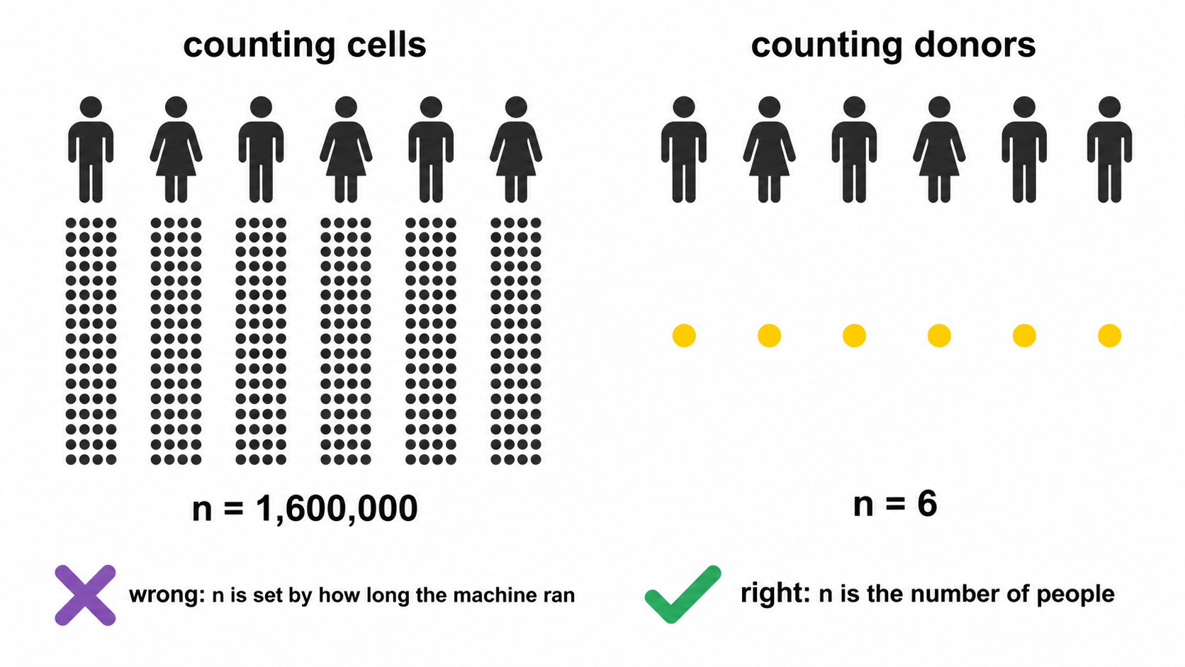
2. Test selection

Group comparisons use Wilcoxon rank-sum and Kruskal-Wallis, which assume independence and ordinal comparability.

The principal alternative, implemented in diffcyt, is limma’s moderated t, which stabilises variance estimates through an empirical Bayes prior shared across markers. At mass cytometry marker counts of 30 to 40 and designed sample sizes, this is the more powerful choice.

At a dozen markers and single-digit donors per group the prior is estimated from too few markers to stabilise, and the normality assumption becomes load-bearing at precisely the sample size where it cannot be assessed.

Cost. Reduced power under normality, and no direct mechanism for covariate adjustment.

Revisit at. Approximately fifteen samples per group, where the prior becomes informative and mixed models can accommodate repeated measures.

2a. The parametric tests, and why they are reported separately

Most immunology papers report a t-test or an ANOVA, and a reviewer may ask for one. Declining to compute it does not remove it from the paper; it moves the calculation somewhere with no record of whether its assumptions held.

So parametric_tests.csv carries the parametric equivalent of every comparison, and group_comparison_stats.csv is unchanged. Two files, two answers, and the columns that decide between them sit on the parametric row.

The transform. Frequencies are proportions. They are bounded, their variance depends on their mean, and near 0 or 100 they are strongly skewed, which is exactly where rare populations live. The parametric tests therefore run on the empirical logit, log((p + e) / (1 − p + e)) with e the smallest non-zero proportion so that 0% and 100% stay finite. It is symmetric about 50% and stabilises the variance near 0 and 100%, where the arcsine square root, the older remedy, does not. Group means are reported back on the percentage scale, because a difference in logits means nothing to a reader.

Which test. Two groups give Welch’s t-test, which does not assume equal variances, with Student’s t beside it. Three or more give Welch’s ANOVA with the classical one-way beside it. Welch’s is the default in both cases because equal variance is an assumption, not a property, and the cost of Welch’s when variances happen to be equal is small.

The assumptions, on every row. brown_forsythe_p tests equal variance, using deviations from the median rather than the mean so it does not itself assume normality. shapiro_p tests normality of the within-group residuals, not the pooled values, which are bimodal whenever the groups differ and would fail the test for the wrong reason. assumptions_met combines them and recommended names the test to read.

Post-hoc. With three or more groups, posthoc_tests.csv carries all three standard families: Games-Howell, which uses Welch’s standard error and pair-specific degrees of freedom and so pairs with Welch’s ANOVA; Tukey HSD, which assumes equal variances and pairs with the classical ANOVA; and Dunn, the rank equivalent that follows Kruskal-Wallis. All three are written, adjusted within each family, and the assumption columns say which to read. Choosing after seeing the p-values is the thing this arrangement is designed to make visible.

What is still not here. Mixed models and GLMMs are the right tool for repeated measures and are not implemented; --paired-column with --condition-column covers the two-timepoint case and nothing wider. Beta regression, which models the bounded support directly rather than transforming it, is the better answer at larger sample sizes. Both become worth the dependency at roughly fifteen donors per group.

3. Compositionality

3.1 Constraint

Population percentages within a sample are constrained to sum to 100 and cannot vary independently. A genuine granulocyte expansion mechanically depresses every lymphocyte percentage. Those depressions test significant while absolute lymphocyte counts per microlitre remain unchanged.

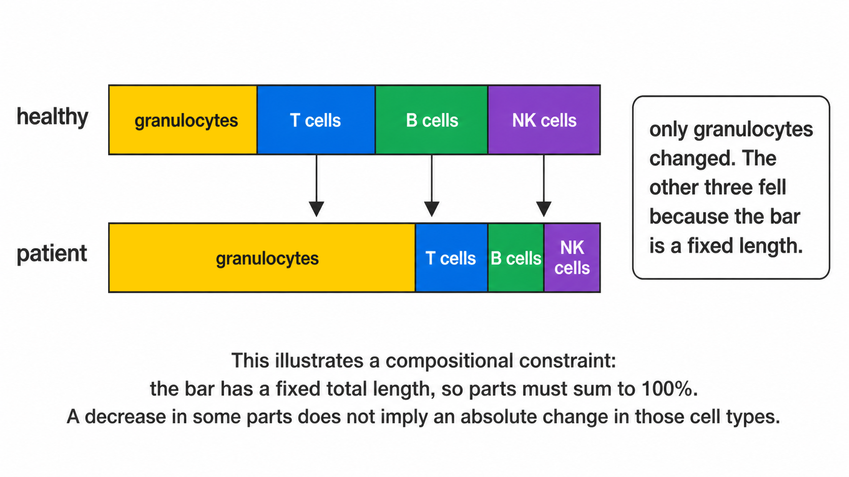
3.2 Log-ratio

clr_frequencies() applies the centred log-ratio, expressing each population relative to the geometric mean of the sample composition rather than to a fixed total.

share <- function() {
  v <- c(60, 25, 15) * exp(rnorm(3, 0, .1))
  100 * v / sum(v)
}
freq <- data.frame(
  sample_id = rep(sprintf("S%02d", 1:6),
                  each = 3),
  population = rep(c("Granulocytes",
                     "CD4 T cells",
                     "B cells"), 6),
  pct_of_cd45_pos =
    as.vector(replicate(6, share())),
  is_control = FALSE, qc_status = "pass")
cl <- clr_frequencies(freq)
head(cl[, c("sample_id", "population",
            "pct_of_cd45_pos", "clr")], 3)

#>   sample_id   population pct_of_cd45_pos
#> 1       S01 Granulocytes        61.69888
#> 2       S01  CD4 T cells        24.02756
#> 3       S01      B cells        14.27356
#>          clr
#> 1  0.8023069
#> 2 -0.1407573
#> 3 -0.6615496

3.3 Concordance

Both parameterisations are tested and compositional_concordance() classifies each result.

robust_to_composition survives both and supports interpretation as an independent change.

raw_only__possible_composition_artefact is significant on percentages and not on log-ratios, which is the configuration produced by section 3.1.

clr_only__was_masked_by_composition is the converse, an independent change obscured by the constraint.

3.4 Limit

The log-ratio does not recover absolute abundance. Proportional expansion of every population leaves the composition invariant and is undetectable in frequency data by construction. Discriminating expansion from relative expansion requires cells per microlitre, so abundance_measure() uses absolute counts wherever the patient table supplies a leukocyte count.

4. Covariates

Age and sex are diagnosed rather than adjusted.

At the sample sizes cytometry cohorts reach, commonly under ten donors per group, a model estimating age and sex effects alongside the group term consumes the residual degrees of freedom required for the comparison of interest. Where the covariate is strongly associated with group, the parameters are not separable at any sample size, because the design contains no observations at the covariate levels required to estimate the effects independently.

stats_confounding() therefore reports the two conditions that jointly define a confounder: differential distribution across groups, and association with the outcome within groups (Rothman, Greenland & Lash 2008), a partial Spearman correlation with group held fixed. stats_rank_ancova() fits the adjusted model on request, labels every row EXPLORATORY, and records NOT FITTED with the reason where residual degrees of freedom are insufficient.

4a. Clinical variables, which are a different question

A confounder is screened to decide whether a group difference can be believed. A clinical variable, a severity score, a laboratory value, an outcome flag, is the question itself, and stats_clinical_association() treats it that way.

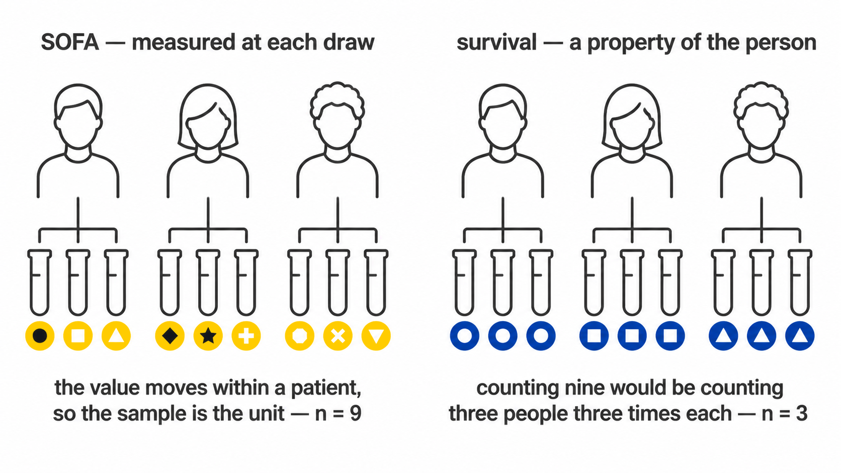
The test follows the variable’s type rather than being chosen:

Variable	Test	Effect reported	Signed
Numeric (SOFA, CRP, lactate, BMI)	Spearman’s rho	rho, with a bootstrap interval	yes
Two levels (28-day survival)	Wilcoxon rank-sum	Cliff’s delta, with a bootstrap interval	yes
Three or more levels (infection focus)	Kruskal-Wallis	epsilon-squared	no

Epsilon-squared is H / (n - 1), the proportion of rank variance the grouping accounts for, bounded 0 to 1. It is unsigned, because a variable with three unordered levels has a magnitude and no direction, and that is carried explicitly in a signed column rather than left for the reader to infer from a sign that happens to be positive. Before it was added, a multi-level variable produced a p-value and nothing else: the figure could say a test had run and not whether it had found anything.

Rank methods throughout, for the reason they are used everywhere else in this package. Clinical scores are ordinal by construction, so a Pearson correlation asserts an interval scale the data does not have. Laboratory values are skewed and carry outliers that are real rather than erroneous, a creatinine of 335 is a patient, not a typing error, and a product-moment correlation on nine points with one such value is a statement about that one patient.

Multiplicity is corrected within each variable, across the populations tested against it. Each variable is one question asked of every population, and that is the family; pooling every variable into one correction would penalise a well-powered variable for the company it keeps. The choice is recorded here because it is a judgement rather than a default.

It also has a stated assumption, which is that the variables are separate questions. They frequently are not: in a cohort where the sickest patients are also the ones who died, SOFA and 28-day survival describe one gradient, and a population associated with both is one finding counted twice. fig_clinical_correlogram() exists to make that visible before the heatmap is read, because no correction can repair it and nothing else in the run would show it. Two-level variables appear there coded 0/1, for which Spearman is the point-biserial correlation of the ranks; variables with three or more unordered levels are excluded rather than coded 1/2/3, which would invent an ordering.

4b. Effect intervals on a small cohort

Every signed effect above is written with a 95% percentile bootstrap interval: 2000 resamples of the patient-value pairs for Spearman, stratified within each arm for Cliff’s delta, from a fixed seed so a given table always yields the same interval and the RNG stream is restored afterwards so nothing downstream is perturbed.

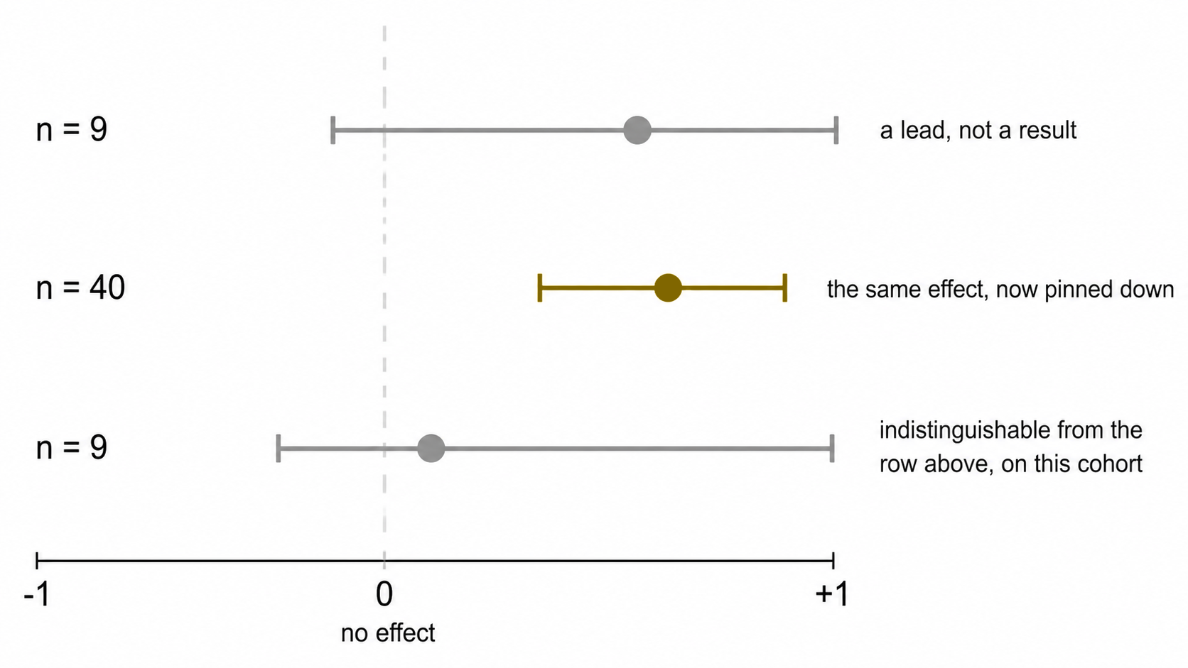
The interval is the part of the answer that carries how little a small cohort constrains the effect. On ten patients a rho of 0.61 with an interval from -0.1 to 0.9 and a rho of 0.05 can be the same underlying quantity, and the point estimate alone cannot say so; reporting the effect and its interval beside the p-value, rather than the p-value alone, is the standard recommendation for exactly this situation.

Its own limits are stated on the figure that draws it. A percentile bootstrap at this sample size is approximate: below about nine observations the effective resample is smaller than the nominal one and coverage falls short of 95%. So a wide interval should be read as this cohort does not constrain the effect rather than as a calibrated range, and no interval is written at all below six samples, a number quoted at a width nobody should trust is worse than a blank.

The same reasoning is why group_differences.png draws the smallest p-value the design can reach. A Wilcoxon rank-sum test has choose(n1 + n2, n1) equally likely rank arrangements under the null, so the most extreme separation possible gives a two-sided p of 2 / choose(n1 + n2, n1). At 4 against 5 that is 0.016, and after correcting across a dozen populations nothing can reach 0.05 however cleanly the groups separate. Where that floor sits above the 0.05 line, an empty region of the figure is a fact about the design and not about the biology.

Two boundaries. This is association, not survival analysis: a 28-day flag is tested as the two-group comparison it is, and no time-to-event model is fitted, because the sample sheet carries no follow-up time and a proportional-hazards fit on a binary column with no time is a category error rather than an approximation. And every test runs on one value per sample, so the replicates are subjects; correlating a score against pooled events would treat one deeply acquired patient as tens of thousands of independent observations, which is the same failure abundance_measure() exists to prevent.

The underpowered column marks every test run on fewer than ten samples. At that size a rank test detects only very large effects, so a null result carries almost no information and should not be reported as evidence of no association.

5. Batch effects

Correction methods displace cells until batch labels mix. This is valid when batch is independent of the study design.

Clinical cohorts rarely satisfy that condition: recruitment and acquisition are typically sequential, so batch and group approach collinearity. Displacing cells until batches mix then also removes the biological contrast, and the algorithm cannot distinguish the two contributions.

batch_mixing_report() returns both required quantities before any correction: iLISI against a permutation null, establishing whether batch structure exists, and Cramér’s V, establishing whether it is separable from group. A high V means no setting makes correction safe, which is the most informative result the diagnostic can return.

--correct-batch performs the correction and is refused above a configurable threshold.

6. Multiplicity

Benjamini-Hochberg correction is applied within each test family, with raw and adjusted p-values both reported.

Differential state adjusts within each measure rather than across both. Median intensity and percent positive are two summaries of the same events and are strongly correlated; pooling them would inflate the family with non-independent hypotheses and over-penalise every result.

7. Effect sizes

Every p-value is reported with an effect size: Cliff’s delta across samples, or matched-pairs rank-biserial for paired designs. Clinical associations add a bootstrap interval on the effect as well; see §4b for why, and for why the interval is suppressed rather than narrowed below six samples.

Differences rather than ratios are reported for transformed intensities. Arcsinh and logicle scales admit negative values, on which a ratio is undefined in interpretation and changes sign without a corresponding change in biology.

8. Measurement resolution

An effect size states how large a difference is relative to the spread between donors. It does not state whether the instrument and the gating strategy could resolve a difference of that size at all.

difference_over_gate_u supplies the second quantity: the observed difference in medians divided by the typical within-sample uncertainty on the frequency, itself propagated from where the thresholds were placed. Below one, the groups differ by less than the distance the cut travels under resampling of the cells that determined it.

This is a screen, not a test. The uncertainty is partly shared across the run, since every sample passes through one panel, one transform and one placement rule, so it cancels in part when a difference is taken and the ratio is conservative. A ratio below one is a reason to open threshold_uncertainty.csv before interpreting the comparison, not grounds to discard it.

difference_over_total_u repeats the comparison against the gate term and the counting term together. The two ratios coincide for an abundant population and separate for a rare one, where the threshold can be well placed and the frequency still rest on too few events to support the difference being tested. Where they disagree, the smaller is the one to act on.

The order to read remains: adjusted p, then effect size, then these. A result that survives all of them is one where the groups differ, the difference is large relative to donor variation, and it is larger than both the distance the gate can move and the noise in the count.

8a. Detection limits

An effect size and a p-value can both be computed from a population of nine events. Neither reports that fact.

detection in population_frequencies.csv classifies each value against the conventional limits of detection and quantification, twenty and fifty events against the parent gate. A population below the limit of quantification in most samples should not be carried into a group comparison at all: the test will run, and its result is a statement about acquisition depth.

This is a screen on the measurement rather than a correction to the test. No p-value is adjusted by it, and the tests behave as they did before.

9. Summary

Question	Function	Unit
Did population abundance change?	stats_group_comparison()	sample
Does it survive the compositional constraint?	clr_frequencies(), compositional_concordance()	sample
Did marker expression change within a population?	stats_marker_state()	sample
Is the contrast confounded by age or sex?	stats_confounding()	sample
Is the contrast confounded by batch?	batch_mixing_report()	cell, descriptive
Is the contrast an artefact of the gate?	stats_threshold_drift(), cluster_gate_agreement()	sample and cell
Is the difference bigger than the gate’s own uncertainty?	run_gate_uncertainty(), annotate_gate_uncertainty()	sample
Were enough cells counted for the frequency to mean anything?	counting_uncertainty()	sample
Which markers shift within a subcluster?	stats_subcluster_shifts()	cell, no p-value

10. Sources for the tests implemented here

Where each method came from, and what it is for.

Proportions. Population frequencies are bounded and their variance depends on their mean, so a test assuming constant variance is wrong in a way that gets worse as the population gets rarer. The logit is used here: Warton and Hui (2011, Ecology 92:3) argue the arcsine square root should not be used for proportions, and for flow cytometry results the logit gives symmetric distributions and homogeneous variances near 0 and 100% (Seiffert et al. 2024, Front Mol Biosci 11:1335174).

Unequal variance. Welch’s t-test and Welch’s ANOVA do not assume equal variances, so they stay valid when group sizes and spreads differ, which they almost always do in an immunophenotyping cohort. Games-Howell is the post-hoc test that matches: it uses Welch’s standard error and pair-specific degrees of freedom rather than one pooled estimate (rstatix).

Rank post-hoc. Dunn’s test compares mean ranks computed over the whole dataset, which is what makes it the correct follow-up to Kruskal-Wallis. A set of pairwise Wilcoxon tests re-ranks within each pair and answers a different question.

Clinical associations: the unit of analysis. A cohort sampled at several timepoints carries two kinds of clinical column. One is constant within a patient , 28-day survival, BMI, age, and asks a between-subject question; the other varies within a patient, a severity score at each draw, and asks a within-subject one. Treating repeated samples from one patient as independent observations is pseudoreplication: it inflates the apparent sample size, narrows the interval and makes significance more likely without a single extra patient having been recruited, and it is common enough in the life sciences to be one of the standard threats to reproducibility (The problem of pseudoreplication in neuroscientific studies, BMC Neuroscience; Statistics Done Wrong, on pseudoreplication). Collapsing to one value per subject is the first remedy named in that literature and is what clin_variable_unit() triggers for a patient-constant column.

For a column that varies within a patient, collapsing would delete the variation being asked about, so the per-sample test is kept and n_patients and repeated_measures are reported beside it. The dedicated method there is a repeated-measures correlation, which estimates the common within-individual slope without averaging (Bland & Altman 1995; Bakdash & Marusich, Frontiers in Psychology 2017, implemented in rmcorr). It is named rather than implemented, for the same reason as the mixed models below.

Effect sizes with intervals, not p-values alone. Reporting the estimated effect with a confidence interval, rather than a p-value on its own, is what the reporting guidelines for prognostic marker studies ask for, and the surveys behind those guidelines found 96% of papers reporting p-values against 42% reporting an interval (REMARK explanation and elaboration, BMC Medicine 2012). clinical_association.csv carries ci_low and ci_high on every signed effect for that reason, and fig_clinical_forest() draws them.

Rank effect sizes. Cliff’s delta is the non-parametric two-group effect size for ordinal or non-normal data, and percentile bootstrap intervals are the standard way to bound it (Cliff’s Delta Calculator, Universitas Psychologica). Epsilon-squared, H / (n - 1), is the corresponding effect size for Kruskal-Wallis, following Tomczak & Tomczak’s recommendation as implemented in rstatix::kruskal_effsize(); it is unsigned because a variable with three unordered levels has no direction. The bootstrap’s own limit at these sample sizes, an effective resample smaller than the nominal one, and coverage falling short of 95% below about nine observations, is documented rather than ignored (Statistical uncertainty analysis for small-sample, high log-variance data), which is why no interval is written below six.

What is not implemented. Generalised linear mixed models are the right tool when donors contribute several samples, and CytoGLMM implements them for cytometry specifically (Seiler et al.). Beta regression models bounded support directly instead of transforming it (npj Systems Biology, 2025). Both need more donors per group than the cohorts this package is aimed at, and both add a dependency whose failure modes are harder to explain than the tests above. --paired-column with --condition-column covers the two-timepoint case; anything wider belongs in one of those packages.

Using cyRAVEN with cyCONDOR

cyRAVEN applies a declared specification and tests whether it held. cyCONDOR clusters events and assigns identity afterwards. The two approaches carry non-overlapping failure modes, which makes combined application informative for a substantial class of study designs.

1. Rationale

Supervised quantification is bounded by its specification. A population absent from the declaration cannot be recovered, because no gate exists to fail.

Unsupervised partitioning carries the complementary limitation. It returns clusters for any input and holds no prior claim capable of being contradicted, so it cannot identify a mis-specified threshold. Its own parameters, cluster count, feature set and transform, are selected after inspecting the data, which relocates analyst discretion rather than removing it.

Applied together, each constrains the other. The principle is established: DAFi converts a manual gating strategy into constraints on a recursive clustering and recovers rare populations that neither approach resolves independently (Lee et al., 2018).

2. Selection

Objective	Tool	Basis
Abundance of a declared population between groups	cyRAVEN	Populations defined a priori, donor-level inference
Verification that gates transferred across samples	cyRAVEN	Threshold drift, phenotype concordance, gate-cluster concordance
Detection of an undeclared population	Both	cyRAVEN identifies the discordance, cyCONDOR characterises the population
Conversion of a cluster into executable gate geometry	cyRAVEN	--explain-clusters, or --external-labels for a labelling cyCONDOR produced
Whether that gate works on the next donor	cyRAVEN	Leave-one-donor-out refitting
A gate file the instrument or Cytobank can read	cyRAVEN	--export-gates, Gating-ML 2.0 in linear units
How precisely a reported frequency is determined	cyRAVEN	Threshold resampling propagated to the population
Differentiation trajectory	cyCONDOR	Diffusion maps and Slingshot
Label transfer to an independent cohort	cyCONDOR	Trained classifiers
Ingestion of existing FlowJo gates	cyCONDOR	.wsp workspace parsing
Data-determined cluster count	cyCONDOR	Phenograph
Unsupervised discovery without leaving cyRAVEN	cyRAVEN	--explore, over every eligible channel, with clusters named from per-sample thresholds. See Explore mode
Whether batch correction is admissible	cyRAVEN	Cramér’s V refusal rule

3. Applications

3.1 Abundance change

A declared population differs in frequency between groups. Four outputs determine whether the difference is interpretable, read in order.

threshold_drift_stats.csv. A flagged marker means the per-sample thresholds separate by group, so the population is not identically defined across the comparison and the difference is partly definitional.

compositional_concordance.csv. Percentages are constrained to sum to 100. A result classified raw_only__possible_composition_artefact is consistent with expansion elsewhere in the composition rather than change in the population tested.

cluster_gate_agreement_populations.csv. A declared population distributed across several clusters is phenotypically heterogeneous, and the aggregate frequency averages subsets that may respond in opposite directions.

confounding_diagnostics.csv. Whether a covariate both differs between groups and associates with the outcome.

cyCONDOR contributes nothing here unless the third output indicates heterogeneity, in which case the constituent subsets require characterisation.

3.2 Undeclared population

Order matters in this analysis.

Run cyRAVEN with --cluster --explain-clusters. Gate-cluster concordance identifies a cluster dominated by the unassigned label, which establishes that the specification is incomplete. cluster_gate_proposals.csv returns two-marker gate geometry selecting those events, with performance measured on held-out cells, which is sufficient to reproduce the gate at the instrument.

Characterise in cyCONDOR. plot_marker_ridgeplot, plot_marker_violinplot and plot_marker_dotplot resolve the full intensity distribution rather than a median, and plot_marker_group_HM compares it across groups. Where the population may occupy a differentiation axis, runDM and runPseudotime establish whether a trajectory is supported.

Return to cyRAVEN. Add the population to the populations: block using the markers the proposal identified and re-run. It now carries a per-sample frequency and a donor-level test.

The final step is not optional. A population identified by clustering and tested by clustering on the same events was selected because it separated in those samples. Once declared, it is tested honestly in the next cohort.

3.3 A cyCONDOR cluster made executable

The reverse direction, and the one that closes the loop. cyCONDOR finds a population; the finding lives in a vector of cluster assignments and cannot be sorted on, drawn at the instrument, or applied to next year’s files without clustering them again.

Export the assignment with the sample and the event index, then hand it over.

fs <- condor@clustering$FlowSOM
meta <- fs$metacluster
cl <- data.frame(
  sample  = condor@anno$sample_id,
  event   = condor@anno$event_index,
  cluster = paste0("k", meta))
write.csv(cl, "labels.csv",
          row.names = FALSE)

--external-labels labels.csv --export-gates

cyRAVEN fits a sequence of two-marker polygon gates to each label, then refits the whole sequence with one donor withheld and scores it on that donor, once per donor. gate_transferability_summary.csv carries the spread of those scores. Read f1_min: a gate that works on nine donors and fails on the tenth has the same median as one that works on all ten.

--export-gates writes the surviving strategy as Gating-ML 2.0 in the linear units the FCS file stores, which Cytobank and FlowRepository read directly and FlowJo reads through an ACS archive.

The join is on sample and event index, never row position. cyCONDOR subsamples at prep_fcd(max_cell = ) and cyRAVEN takes its own cap for the embedding, so the two tables are not row-aligned and a positional join would relabel every cell without raising anything.

Hypergate established cluster-to-gate conversion, fitting one hyperrectangle per cluster (Becht et al., 2018). What is added here is the polygon hierarchy, which is the shape a sorter is actually driven in, the per-donor score distribution, and the gate file.

3.4 Multi-site or longitudinal designs

Analyst variance is the limiting factor. Thirty-eight operators gating the same files carried a median expanded uncertainty of 3.6% under a gauge repeatability and reproducibility design (Grant et al., 2021), and across 320 routine clinical samples the residual dispersion was structured primarily by operator identity rather than by instrument configuration (Mead et al., 2026). Reagent standardisation alone is insufficient: EuroFlow reached between-centre coefficients of variation below 7% only after standardising the analysis (Kalina et al., 2012).

Use cyRAVEN as the primary analysis. A declared specification with per-sample thresholds removes the analyst from the step at which that variance enters. Version-control the config alongside the results and retain run_manifest.txt.

Write a baseline from the first accepted run and pass --baseline on every later one. The within-run threshold check compares each sample against its peers, which finds a bad tube and cannot find a site or a season that moved as a whole, since the peer median moves with it. On a scheduled pipeline, --fail-on-drift makes the verdict an exit code.

Use cyCONDOR as a periodic audit. Cluster the accumulated data without reference to the specification and confirm that reported populations still resolve as coherent clusters. Populations that begin to split or merge indicate acquisition drift requiring the specification to be revisited.

4. Execution

Both tools read the same FCS files. cyCONDOR requires an annotation table whose first column names the files, which is the information a cyRAVEN sample map already carries, so one file serves both.

run_cyraven(list(
  dir = "data/fcs/",
  outdir = "results_cyraven/",
  sample_map = "data/sample_map.csv",
  config = "data/panel.yaml",
  group_column = "cohort",
  reference_group = "Healthy controls",
  unsupervised = TRUE,
  explain_clusters = TRUE
))

anno <- read.csv("data/sample_map.csv")
at <- "results_condor/anno_table.csv"
write.csv(anno, at, row.names = FALSE)

condor <- cyCONDOR::prep_fcd(
  data_path = "data/fcs/",
  max_cell = 30000, useCSV = FALSE,
  transformation = "auto_logi",
  remove_param = c("Time", "InFile"),
  anno_table = at,
  filename_col = "file", seed = 42)
condor <- cyCONDOR::runPCA(
  condor, data_slot = "orig", seed = 42)
condor <- cyCONDOR::runUMAP(
  condor, input_type = "pca",
  data_slot = "orig", seed = 42)
condor <- cyCONDOR::runFlowSOM(
  condor, input_type = "pca",
  data_slot = "orig",
  nClusters = 8, seed = 42)

The benchmark/ directory of the cyRAVEN repository executes both on a public dataset and writes the comparison.

5. Embeddings

The two UMAPs are not comparable, for four reasons measured on the benchmark dataset and given in order of magnitude.

Event set. cyCONDOR embeds all 235,259 events. cyRAVEN embeds 40,000 events surviving scatter, singlet, viability and CD45 gating. A fraction of the cyCONDOR manifold is debris.

Feature set. cyCONDOR includes FSC-A, FSC-H, FSC-W and SSC-A among eleven features. Scatter spans decades and dominates the principal components on which the embedding is computed, so much of the resulting structure reflects size and granularity. cyRAVEN uses scatter for gating and excludes it from the feature set, embedding four markers.

Input space. cyCONDOR embeds principal component scores; cyRAVEN embeds the scaled marker matrix, which alters the neighbour graph before construction.

Transform. Auto-logicle per file against arcsinh pooled per panel places identical raw intensities at different coordinates.

Compare the tables, not the figures.

6. Resolution

Cluster count is an analytical choice with consequences. On the benchmark data FlowSOM requested at 8 returns 8 clusters; Phenograph, which determines its own, returns 24 on the same events. Both are correct implementations. Neither corresponds to the number of populations present.

A result that appears at one resolution and disappears at another is a property of the setting. Confirm persistence across resolutions before interpretation.

FlowSOM is a defensible default: it ranked at or near the top across every dataset in the reference comparison of clustering methods, at runtimes permitting routine use as a cross-check (Weber and Robinson, 2016).

7. References

• Lee et al., 2018. DAFi: gating strategy as constraint on recursive clustering. Cytometry A.
• Briefings in Bioinformatics, 2025. Systematic comparison of manual gating, unsupervised clustering and auto-gating across 23 tools.
• Weber and Robinson, 2016. Clustering method comparison. Cytometry A 89:1084.
• Kalina et al., 2012. EuroFlow standardisation. Leukemia 26:1986.
• Grant et al., 2021. Operator subjectivity as measurement uncertainty: 38 participants, median expanded uncertainty 3.6%. PDA J Pharm Sci Technol 75:33.
• Mead et al., 2026. Interpretive contribution to analytical variability, 320 clinical samples and six technologists. Cytometry B Clin Cytom.
• Becht et al., 2018. Hypergate: reverse-engineering a gating strategy from a cluster. Bioinformatics 35:301.
• Spidlen et al., 2015. ISAC Gating-ML 2.0. Cytometry A 87:683.
• Grant et al., 2021. Uncertainty analysis applied to manual gating; a diagrammatical protocol cut between-participant variation by 57%. Methods Protoc 4:24.

Driving it from Claude Code

The repository ships a skill for Claude Code at .claude/skills/cyraven/. Installed, it gives the assistant the parts of this documentation that determine whether an answer is correct: Docker as the execution path, the gate hierarchy and specification syntax, and the order in which the outputs must be read.

It is documentation, not a wrapper. Nothing about the pipeline changes, and every command works without it.

The skill executes through Docker by default and does not fall back to a local R installation unless the user states that Docker is unavailable, for the reproducibility reasons given in the README.

1. What it covers

File	Content
SKILL.md	What cyRAVEN does, the Docker execution commands, required inputs, the flags that matter, and the analytical constraints in section 4
references/docker.md	Build and run in detail, path and mount semantics, Windows and PowerShell, resource tuning, iterating with CYRAVEN_SOURCE, container-specific failures
references/gating.md	The four-gate hierarchy, per-sample thresholding and the source column, writing the population YAML, three-level markers, arcsinh against logicle, compensation
references/interpretation.md	Every output file and the order to read them in, with the columns that decide whether a result stands
references/troubleshooting.md	Failure modes with their actual causes

Only SKILL.md is read when the skill activates. The reference files are opened when the task needs them, so the description above is also the routing table.

2. Installing

For every project

Copy the directory into the personal skills folder:

cp -r .claude/skills/cyraven \
  ~/.claude/skills/

Copy-Item -Recurse `
  .claude\skills\cyraven `
  $HOME\.claude\skills\

Confirm with /skills, or ask Claude to invoke /cyraven.

For this repository only

Nothing to do. A checkout already contains .claude/skills/cyraven/, and Claude Code discovers it when the session is rooted in the repository.

Without a copy

Point Claude at the raw SKILL.md by pasting its link with:

Read this SKILL.md and follow it:
<paste the link here>

3. Using it

The skill activates on its own when a request matches its description. Force it with /cyraven.

Requests it is built for:

Run cyRAVEN on the FCS files in ./data.
The panel is CD3, CD4, CD8, CD14, CD16,
CD19, CD56, HLA-DR.

Set up the demonstration dataset and
show me what the output looks like.

Write a population spec for this panel
and explain each definition.

My frequency table came out empty. Why?

Read results/ and tell me which findings
survive.

Is the difference in CD8 T cells between
the two cohorts real?

The first builds and invokes the container without being asked to, because that is the skill’s default execution path.

The last is the case worth having the skill for. It has a documented answer that is not a p-value: adjusted p, then Cliff’s delta, then difference_over_gate_u, then difference_over_total_u, then a check that the marker is not flagged in threshold_drift_stats.csv. The order is set out in Statistics §8, and the skill states it so the assistant does not stop at the first significant result.

4. Analytical constraints

The skill carries five positions the tool takes. They are recorded because overriding any of them produces output that appears correct and is not. Each is documented at length elsewhere and summarised there only to the extent needed to apply it.

Constraint	Treated in full
Thresholds are not transferred between samples	Gating §2.1
count is an event count, not a cell number	Output §4
Placement precision does not imply counting sufficiency	Gating §2.5
A specification is a hypothesis, not a validated result	Diagnostics
Gates are inspected before any derived number is quoted	Diagnostics §1

5. Contributing through it

SKILL.md also carries the conventions this package is maintained under, so a change proposed with the skill loaded arrives in the right shape:

• Additions are additive. Every file the previous version wrote is still written, with the same name, the same columns in the same order, and the same values.
• Additivity is verified by running both versions on one cohort and comparing byte for byte, not by asserting it.
• Anything that only adds an output is on by default. Anything that changes an existing number is opt-in.
• Any new entry point that consumes random draws saves and restores .Random.seed. run_cyraven() seeds once and the UMAP cell selection draws from that stream, so a step that spends draws silently redraws every embedding in the run.

6. Keeping it accurate

The skill quotes flag defaults, output filenames and column names. Those were checked against the source when it was written and will drift if the package changes without it.

When adding a flag or an output, update SKILL.md and the reference file that mentions the area. The filenames are verifiable mechanically:

grep -rohE \
  '"[a-z0-9_]+\.(csv|png|txt|rds)"' \
  R/pipeline.R | sort -u

Cross-check that list against references/interpretation.md.